
Direct LiNGAM assumes that observations are independent and
identically distributed (i.i.d.), a requirement that time
series data violate. This article covers the two time-series methods in
lingamr:
-
VAR-LiNGAM (
lingam_var()): stationary time series whose temporal dependence is captured by an autoregressive (AR) part. -
VARMA-LiNGAM (
lingam_varma()): time series whose disturbances also have a moving-average (MA) part, so past shocks influence the present.
If your data are i.i.d. cross-sectional observations, start with the Direct LiNGAM article instead. For an overview of all methods, see the method selection guide.
VAR-LiNGAM: Causal Discovery in Time Series
VAR-LiNGAM (Hyvärinen et al., 2010) handles stationary time series by first fitting a Vector Autoregression (VAR) model to absorb temporal autocorrelation, then applying Direct LiNGAM to the VAR residuals to recover the instantaneous causal structure . The model is:
where encodes contemporaneous causal effects (strictly acyclic), encode lagged effects, and are mutually independent non-Gaussian disturbances.
Sample Data
generate_varlingam_sample() produces a three-variable
time series from a VAR(1)-LiNGAM model. The instantaneous structure is
(coefficients 0.6 and −0.5), and the only cross-variable lag-1 effect is
(coefficient 0.3).
s <- generate_varlingam_sample(n = 1000, seed = 42)

# True instantaneous coefficient matrix B0  (B0[i, j]: x_j -> x_i)
s$true_B0
#>      [,1] [,2] [,3]
#> [1,]  0.0  0.0    0
#> [2,]  0.6  0.0    0
#> [3,]  0.0 -0.5    0

# True lag-1 coefficient matrix  (M1[i, j]: x_j(t-1) -> x_i(t), structural)
s$true_M1
#>      [,1] [,2] [,3]
#> [1,]  0.4  0.0  0.3
#> [2,]  0.0  0.3  0.0
#> [3,]  0.0  0.0  0.5
Fitting VAR-LiNGAM
Pass the data matrix to lingam_var(). Rows must be in
chronological order (earliest first).
model <- lingam_var(s$data, lags = 1)
model
#> VAR-LiNGAM Result
#>   Variables : 3
#>   Lag order : 1
#>   Causal order (instantaneous): x0 -> x1 -> x2
#>
#> Instantaneous adjacency matrix B0 (row = to, col = from):
#>       x0     x1 x2
#> x0 0.000  0.000  0
#> x1 0.576  0.000  0
#> x2 0.000 -0.491  0
#>
#> Lagged adjacency matrix B1 (row = to, col = from):
#>     x0    x1    x2
#> x0 0.4 0.000 0.309
#> x1 0.0 0.225 0.000
#> x2 0.0 0.000 0.495
The result object contains adjacency_matrices, a
three-dimensional array of shape
[1 + lags, n_features, n_features]:
-
[1, , ]("lag0"): instantaneous matrix .B0[i, j]is the direct effect of on at the same time step. -
[k + 1, , ]("lagk"): lagged matrix .Bk[i, j]is the direct structural effect of on .
Both can be extracted by their dimension label:
B0 <- model$adjacency_matrices["lag0", , ]
B1 <- model$adjacency_matrices["lag1", , ]

round(B0, 2)  # compare with s$true_B0
#>      x0    x1 x2
#> x0 0.00  0.00  0
#> x1 0.58  0.00  0
#> x2 0.00 -0.49  0
round(B1, 2)  # compare with s$true_M1
#>     x0   x1   x2
#> x0 0.4 0.00 0.31
#> x1 0.0 0.23 0.00
#> x2 0.0 0.00 0.50
Lag Order Selection
By default, lingam_var() automatically selects the lag
order among 1:lags using the Bayesian Information Criterion
(criterion = "bic"). The alternatives "aic",
"hqic", and "fpe" are also supported. To use a
fixed lag order without automatic selection, set
criterion = NULL:
# Fix lag order to 2 without IC-based selection
model_lag2 <- lingam_var(s$data, lags = 2, criterion = NULL)
Stationarity Check
VAR-LiNGAM is defined for stationary processes.
check_var_stationarity() inspects the eigenvalues of the
VAR companion matrix: the process is stationary when all moduli are
strictly less than 1.
check_var_stationarity(model)
#> === VAR Stationarity Check ===
#> Lag order:         1
#> Max |eigenvalue|:  0.4942  (threshold 1.00)
#> Stationary:        YES
A max_modulus at or above 1 indicates a unit-root or
explosive process. In that case, differencing the series before analysis
is recommended.
Residual Diagnostics
LiNGAM assumes that the error terms
are non-Gaussian.
test_varlingam_residual_normality() tests whether the
LiNGAM innovations
(where
are the stored VAR residuals) depart from normality. A small p-value
(reject
:
Gaussian) supports the model assumption.
test_varlingam_residual_normality(model)
#> === Residual Normality Test ===
#> Method:         shapiro
#> Sample size:    999
#> Significance:   0.050
#> Non-Gaussian:   3 / 3 variables
#>
#>  variable statistic   p_value is_non_gauss skewness kurtosis
#>        x0    0.9498 < 2.2e-16         TRUE    0.088   -1.220
#>        x1    0.9536 < 2.2e-16         TRUE   -0.007   -1.238
#>        x2    0.9518 < 2.2e-16         TRUE   -0.046   -1.221
#>
#> Interpretation:
#>   is_non_gauss = TRUE  -> rejects normality (supports LiNGAM assumption)
#>   is_non_gauss = FALSE -> cannot reject normality (LiNGAM may not fit)
#>
#> All residuals are non-Gaussian. LiNGAM assumption is supported.
test_varlingam_residual_normality_all() runs several
tests at once and appends skewness and excess kurtosis columns for a
quick overview:
test_varlingam_residual_normality_all(model, methods = c("shapiro", "jb"))
#> Registered S3 method overwritten by 'quantmod':
#>   method            from
#>   as.zoo.data.frame zoo
#>   variable     skewness  kurtosis    p_shapiro         p_jb all_non_gauss
#> 1       x0  0.088013433 -1.219504 6.041150e-18 1.898481e-14          TRUE
#> 2       x1 -0.007060832 -1.238431 3.114110e-17 1.365574e-14          TRUE
#> 3       x2 -0.046381574 -1.220525 1.452023e-17 2.864375e-14          TRUE
plot_varlingam_residual_qq() draws per-variable normal
Q-Q plots. Deviations from the straight reference line indicate
non-Gaussianity.
plot_varlingam_residual_qq(model)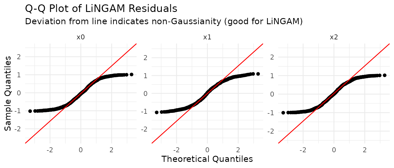
Total Causal Effects
estimate_var_total_effect() estimates the
total causal effect of one variable on another,
integrating over all direct and mediated paths. The
from_lag argument controls the time offset of the cause:
from_lag = 0 (default) gives the contemporaneous total
effect; from_lag = 1 gives the one-step-ahead effect of
on
.
# Total effect x0 -> x2 (contemporaneous)
estimate_var_total_effect(s$data, model, from_index = 1, to_index = 3)
#> [1] -0.2582049

# Total effect x0(t-1) -> x2(t) (one-step-ahead)
estimate_var_total_effect(s$data, model, from_index = 1, to_index = 3, from_lag = 1)
#> [1] -0.2752551
Variable indices are 1-based integers, or column names as character strings.
Bootstrap
lingam_var_bootstrap() quantifies the uncertainty of the
estimated structure by re-running VAR-LiNGAM on residual
bootstrap samples. Unlike the Direct LiNGAM bootstrap (which
resamples i.i.d. rows), VAR-LiNGAM holds the fitted values fixed and
resamples only the VAR residuals, preserving the temporal structure of
the series.
bs_var <- lingam_var_bootstrap(
  s$data,
  n_sampling = 100L,
  seed       = 42,
  verbose    = FALSE
)
get_var_probabilities() returns the proportion of
bootstrap samples in which each directed edge was detected. The column
layout mirrors adjacency_matrices: the first
n_features columns correspond to the instantaneous
structure (lag 0), the next n_features to lag 1, and so
on.
round(get_var_probabilities(bs_var), 2)
#>      [,1] [,2] [,3] [,4] [,5] [,6]
#> [1,] 0.00    0    0 1.00    0 1.00
#> [2,] 1.00    0    0 0.01    1 0.01
#> [3,] 0.02    1    0 0.00    0 1.00
get_var_paths() enumerates all causal paths between two
variables found across bootstrap samples, together with each path’s
average total effect and detection probability.
# Paths from x0 to x2 at the same time step (from_lag = 0)
get_var_paths(bs_var, from_index = 1, to_index = 3)
#>      path      effect probability
#> 1 1, 2, 3 -0.28289316        1.00
#> 2    1, 3  0.08085689        0.02
# Paths from x0(t-1) to x2(t)  (from_lag = 1)
get_var_paths(bs_var, from_index = 1, to_index = 3, from_lag = 1)
#>            path       effect probability
#> 1    4, 1, 2, 3 -0.112845948        1.00
#> 2    4, 5, 2, 3 -0.062338986        1.00
#> 3  4, 5, 6,....  0.024970830        1.00
#> 4    4, 5, 6, 3 -0.139242633        1.00
#> 5       4, 1, 3  0.034930592        0.02
#> 6  4, 5, 6,.... -0.007793044        0.02
#> 7  4, 6, 1,.... -0.007793044        0.02
#> 8    4, 6, 1, 3  0.002044126        0.02
#> 9       4, 6, 3  0.040411503        0.02
#> 10      4, 2, 3 -0.068176510        0.01
#> 11 4, 5, 6,.... -0.018273144        0.01
VARMA-LiNGAM: Time Series with Moving-Average Errors
VARMA-LiNGAM (Kawahara et al., 2011) extends
VAR-LiNGAM with a moving-average (MA) part: the model is
,
so past disturbances can influence the present alongside the lagged
variables. lingam_varma() estimates the reduced-form VARMA
coefficients by the deterministic two-stage Hannan-Rissanen procedure
(the Python reference uses state-space maximum likelihood), applies
Direct LiNGAM to the residuals, and returns the AR-side matrices
psis (with psis[1, , ] = B0) and the MA-side
matrices omegas.
s_varma <- generate_varmalingam_sample(n = 1000, seed = 42)
model_varma <- lingam_varma(s_varma$data, order = c(1, 1))
print(model_varma)
#> VARMA-LiNGAM Result
#>   Variables : 3
#>   Order (p, q) : (1, 0)
#>   Causal order (instantaneous): x0 -> x1 -> x2
#>
#> Instantaneous adjacency matrix B0 (row = to, col = from):
#>       x0     x1 x2
#> x0 0.000  0.000  0
#> x1 0.613  0.000  0
#> x2 0.000 -0.474  0
#>
#> Lagged adjacency matrix psi1 (row = to, col = from):
#>        x0    x1     x2
#> x0  0.472 0.000  0.176
#> x1 -0.169 0.350 -0.166
#> x2  0.000 0.216  0.501
check_varma_stationarity() checks the AR eigenvalues
(stationarity) and also the MA eigenvalues (invertibility), which
Hannan-Rissanen does not enforce.
check_varma_stationarity(model_varma)
#> === VARMA Stationarity / Invertibility Check ===
#> Order (p, q):         (1, 0)
#> Max |AR eigenvalue|:  0.5507  (threshold 1.00)
#> Stationary:           YES
#> Max |MA eigenvalue|:  0.0000  (threshold 1.00)
#> Invertible:           YES
Residual Diagnostics
As in VAR-LiNGAM, the error terms are assumed to be
non-Gaussian.
test_varmalingam_residual_normality() tests whether a
VARMA-LiNGAM residual series departs from normality. By default
(on = "innovations") it targets the LiNGAM innovations
,
where
are the stored VARMA residuals; set on = "varma" to test
directly instead. A small p-value (reject
:
Gaussian) supports the model assumption.
test_varmalingam_residual_normality(model_varma)
#> === Residual Normality Test ===
#> Method:         shapiro
#> Sample size:    999
#> Significance:   0.050
#> Non-Gaussian:   3 / 3 variables
#>
#>  variable statistic   p_value is_non_gauss skewness kurtosis
#>        x0    0.9587  3.42e-16         TRUE    0.079   -1.164
#>        x1    0.9561 < 2.2e-16         TRUE    0.007   -1.223
#>        x2    0.9638  4.94e-15         TRUE   -0.050   -1.139
#>
#> Interpretation:
#>   is_non_gauss = TRUE  -> rejects normality (supports LiNGAM assumption)
#>   is_non_gauss = FALSE -> cannot reject normality (LiNGAM may not fit)
#>
#> All residuals are non-Gaussian. LiNGAM assumption is supported.
test_varmalingam_residual_normality_all() runs several
tests at once and appends skewness and excess kurtosis columns for a
quick overview:
test_varmalingam_residual_normality_all(model_varma, methods = c("shapiro", "jb"))
#>   variable     skewness  kurtosis    p_shapiro         p_jb all_non_gauss
#> 1       x0  0.079398790 -1.163565 3.422206e-16 3.425038e-13          TRUE
#> 2       x1  0.006503161 -1.223165 9.881994e-17 2.986500e-14          TRUE
#> 3       x2 -0.050016361 -1.139036 4.944104e-15 1.522893e-12          TRUE
plot_varmalingam_residual_qq() draws per-variable normal
Q-Q plots (the same on argument selects the residual
series). Deviations from the straight reference line indicate
non-Gaussianity.
plot_varmalingam_residual_qq(model_varma)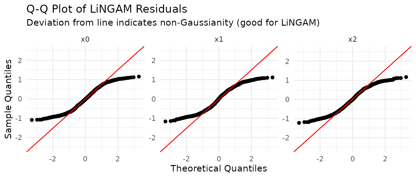
Total Causal Effects
estimate_varma_total_effect() estimates the
total causal effect of one variable on another, the
VARMA-LiNGAM counterpart of estimate_var_total_effect(): it
integrates over both the AR (psi) and MA (omega) structure. As in
VAR-LiNGAM, from_lag = 0 (default) gives the
contemporaneous total effect and from_lag = 1 gives the
one-step-ahead effect of
on
.
# Total effect x0 -> x2 (contemporaneous)
estimate_varma_total_effect(s_varma$data, model_varma, from_index = 1, to_index = 3)
#> [1] -0.2512211

# Total effect x0(t-1) -> x2(t) (one-step-ahead)
estimate_varma_total_effect(s_varma$data, model_varma, from_index = 1, to_index = 3, from_lag = 1)
#> [1] -0.1064222
Bootstrap
lingam_varma_bootstrap(),
get_varma_probabilities(), and
get_varma_paths() mirror their VAR-LiNGAM counterparts,
re-running VARMA-LiNGAM on residual bootstrap samples. In the
probability matrix, the first 1 + p column blocks are the
psi (lag) matrices and the final q blocks are the omega
(MA) matrices.
bs_varma <- lingam_varma_bootstrap(
  s_varma$data,
  n_sampling = 100L,
  order      = c(1, 1),
  criterion  = NULL,
  seed       = 42,
  verbose    = FALSE
)
round(get_varma_probabilities(bs_varma, min_causal_effect = 0.1), 2)
#>      [,1] [,2] [,3] [,4] [,5] [,6] [,7] [,8] [,9]
#> [1,] 0.00    0    0 0.99 0.00 0.93 0.73 0.00 0.00
#> [2,] 1.00    0    0 0.75 1.00 0.84 0.09 0.01 0.06
#> [3,] 0.07    1    0 0.16 0.08 0.89 0.11 0.00 0.99
VAR or VARMA?
- Start with VAR-LiNGAM: it is simpler, faster, and its lag order can be selected automatically by information criteria.
- Switch to VARMA-LiNGAM when the VAR residuals remain autocorrelated even after increasing the lag order — a sign that the disturbances have an MA component that a finite-order VAR can only approximate with many lags.
- Both methods assume stationarity; check with
check_var_stationarity()/check_varma_stationarity(), and difference the series when a unit root is suspected.
Related Articles
- Method selection guide — which method fits your data
- Direct LiNGAM in depth — the i.i.d. building block
- Bootstrap and diagnostics — assessing the reliability of estimated structures