時系列: VAR-LiNGAMとVARMA-LiNGAM

Direct LiNGAMは観測値が独立同一分布（i.i.d.）であることを仮定するが、時系列データはこの要件を満たさない。この記事では lingamr の2つの時系列手法を扱う。

VAR-LiNGAM（lingam_var()）: 時間的依存が自己回帰（AR）部分で表現できる定常時系列。
VARMA-LiNGAM（lingam_varma()）: 撹乱項に移動平均（MA）部分もあり、過去のショックが現在に影響する時系列。

データがi.i.d.のクロスセクション観測なら、まず Direct LiNGAM記事から始めること。全手法の概観は手法選択ガイドを参照。

library(lingamr)

VAR-LiNGAM：時系列データの因果探索

VAR-LiNGAM（Hyvärinen et al., 2010）は、まずベクトル自己回帰（VAR）モデルを当てはめて時間的な自己相関を吸収し、その後VARの残差にDirect LiNGAMを適用することで瞬時因果構造 $B_0$ を復元することで、定常な時系列を扱う。モデルは以下の通りである。

$X_t = B_0\,X_t + \sum_{k=1}^{p} B_k\,X_{t-k} + e_t$

ここで、 $B_0$ は同時点の因果効果（厳密に非巡回）を、 $B_1, \ldots, B_p$ はラグ効果を表し、 $e_t$ は互いに独立な非ガウス擾乱項である。

サンプルデータ

generate_varlingam_sample() は、VAR(1)-LiNGAMモデルから3変数の時系列を生成する。瞬時構造は $x_0 \to x_1 \to x_2$ （係数0.6と−0.5）であり、変数をまたぐラグ1効果は $x_2(t-1) \to x_0(t)$ （係数0.3）のみである。

s <- generate_varlingam_sample(n = 1000, seed = 42)

# True instantaneous coefficient matrix B0  (B0[i, j]: x_j -> x_i)
s$true_B0
#>      [,1] [,2] [,3]
#> [1,]  0.0  0.0    0
#> [2,]  0.6  0.0    0
#> [3,]  0.0 -0.5    0

# True lag-1 coefficient matrix  (M1[i, j]: x_j(t-1) -> x_i(t), structural)
s$true_M1
#>      [,1] [,2] [,3]
#> [1,]  0.4  0.0  0.3
#> [2,]  0.0  0.3  0.0
#> [3,]  0.0  0.0  0.5

VAR-LiNGAMのあてはめ

データ行列を lingam_var() に渡す。行は時系列順（最も古い時点が先頭）である必要がある。

model <- lingam_var(s$data, lags = 1)
model
#> VAR-LiNGAM Result
#>   Variables : 3
#>   Lag order : 1
#>   Causal order (instantaneous): x0 -> x1 -> x2
#> 
#> Instantaneous adjacency matrix B0 (row = to, col = from):
#>       x0     x1 x2
#> x0 0.000  0.000  0
#> x1 0.576  0.000  0
#> x2 0.000 -0.491  0
#> 
#> Lagged adjacency matrix B1 (row = to, col = from):
#>     x0    x1    x2
#> x0 0.4 0.000 0.309
#> x1 0.0 0.225 0.000
#> x2 0.0 0.000 0.495

結果オブジェクトには、[1 + lags, n_features, n_features] の形状を持つ3次元配列 adjacency_matrices が含まれる。

[1, , ]（"lag0"）: 瞬時行列 $B_0$ 。B0[i, j]は、同じ時点における $x_j$ から $x_i$ への直接効果。
[k + 1, , ]（"lagk"）: ラグ行列 $B_k$ 。Bk[i, j]は、 $x_j(t-k)$ から $x_i(t)$ への直接構造効果。

いずれも次元ラベルで取り出せる。

B0 <- model$adjacency_matrices["lag0", , ]
B1 <- model$adjacency_matrices["lag1", , ]

round(B0, 2)  # compare with s$true_B0
#>      x0    x1 x2
#> x0 0.00  0.00  0
#> x1 0.58  0.00  0
#> x2 0.00 -0.49  0
round(B1, 2)  # compare with s$true_M1
#>     x0   x1   x2
#> x0 0.4 0.00 0.31
#> x1 0.0 0.23 0.00
#> x2 0.0 0.00 0.50

ラグ次数の選択

デフォルトでは、lingam_var() はベイズ情報量規準（criterion = "bic"）を用いて 1:lags の中からラグ次数を自動選択する。"aic"、"hqic"、"fpe" にも対応している。自動選択を使わず固定のラグ次数を使うには、criterion = NULL を設定する。

# Fix lag order to 2 without IC-based selection
model_lag2 <- lingam_var(s$data, lags = 2, criterion = NULL)

定常性の確認

VAR-LiNGAMは定常過程を対象に定義される。check_var_stationarity() はVARのコンパニオン行列の固有値を調べる。すべてのモジュラス（絶対値）が厳密に1未満 であれば、過程は定常である。

check_var_stationarity(model)
#> === VAR Stationarity Check ===
#> Lag order:         1
#> Max |eigenvalue|:  0.4942  (threshold 1.00)
#> Stationary:        YES

max_modulus が1以上の場合、単位根過程または発散過程であることを示す。その場合は、分析前に系列を差分することが推奨される。

残差診断

LiNGAMは誤差項 $e_t$ が非ガウスであることを仮定する。 test_varlingam_residual_normality() は、LiNGAMのイノベーション $e_t = (I - B_0)\,n_t$ （ $n_t$ は保存されたVAR残差）が正規性から逸脱しているかを検定する。p値が小さい（ $H_0$ : ガウス、を棄却する）ことは、モデルの仮定を支持する。

test_varlingam_residual_normality(model)
#> === Residual Normality Test ===
#> Method:         shapiro
#> Sample size:    999
#> Significance:   0.050
#> Non-Gaussian:   3 / 3 variables
#> 
#>  variable statistic   p_value is_non_gauss skewness kurtosis
#>        x0    0.9498 < 2.2e-16         TRUE    0.088   -1.220
#>        x1    0.9536 < 2.2e-16         TRUE   -0.007   -1.238
#>        x2    0.9518 < 2.2e-16         TRUE   -0.046   -1.221
#> 
#> Interpretation:
#>   is_non_gauss = TRUE  -> rejects normality (supports LiNGAM assumption)
#>   is_non_gauss = FALSE -> cannot reject normality (LiNGAM may not fit)
#> 
#> All residuals are non-Gaussian. LiNGAM assumption is supported.

test_varlingam_residual_normality_all() は複数の検定を一度に実行し、歪度と尖度（超過尖度）の列を追加して概要を素早く把握できるようにする。

test_varlingam_residual_normality_all(model, methods = c("shapiro", "jb"))
#> Registered S3 method overwritten by 'quantmod':
#>   method            from
#>   as.zoo.data.frame zoo
#>   variable     skewness  kurtosis    p_shapiro         p_jb all_non_gauss
#> 1       x0  0.088013433 -1.219504 6.041150e-18 1.898481e-14          TRUE
#> 2       x1 -0.007060832 -1.238431 3.114110e-17 1.365574e-14          TRUE
#> 3       x2 -0.046381574 -1.220525 1.452023e-17 2.864375e-14          TRUE

plot_varlingam_residual_qq() は変数ごとの正規QQプロットを描画する。直線の基準線からの逸脱は非ガウス性を示す。

plot_varlingam_residual_qq(model)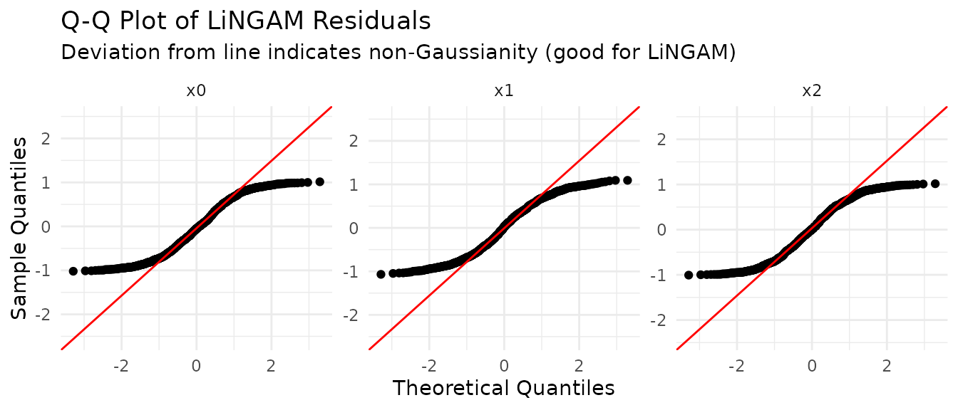

総因果効果

estimate_var_total_effect() は、直接パスとすべての媒介パスを積算することで、ある変数から別の変数への総因果効果を推定する。from_lag 引数は原因の時点オフセットを制御する。from_lag = 0（デフォルト）は同時点の総効果を、from_lag = 1 は $x_j(t-1)$ から $x_i(t)$ への1期先の効果を与える。

# Total effect x0 -> x2 (contemporaneous)
estimate_var_total_effect(s$data, model, from_index = 1, to_index = 3)
#> [1] -0.2582049

# Total effect x0(t-1) -> x2(t) (one-step-ahead)
estimate_var_total_effect(s$data, model, from_index = 1, to_index = 3, from_lag = 1)
#> [1] -0.2752551

変数のインデックスは1始まりの整数、または文字列としての列名で指定する。

ブートストラップ

lingam_var_bootstrap() は、残差ブートストラップのサンプルに対してVAR-LiNGAMを再実行することで、推定構造の不確実性を定量化する。（i.i.d.の行をリサンプルする） Direct LiNGAMのブートストラップとは異なり、VAR-LiNGAMは当てはめ値を固定したまま VAR残差のみをリサンプルし、系列の時間的構造を保持する。

bs_var <- lingam_var_bootstrap(
  s$data,
  n_sampling = 100L,
  seed       = 42,
  verbose    = FALSE
)

get_var_probabilities() は、各有向エッジがブートストラップサンプルの何割で検出されたかを返す。列のレイアウトは adjacency_matrices と対応しており、最初の n_features 列が瞬時構造（lag 0）に、次の n_features 列がlag 1に対応し、以下同様に続く。

round(get_var_probabilities(bs_var), 2)
#>      [,1] [,2] [,3] [,4] [,5] [,6]
#> [1,] 0.00    0    0 1.00    0 1.00
#> [2,] 1.00    0    0 0.01    1 0.01
#> [3,] 0.02    1    0 0.00    0 1.00

get_var_paths() は、ブートストラップサンプル全体から見つかった2変数間のすべての因果パスを、各パスの平均総効果と検出確率とともに列挙する。

# Paths from x0 to x2 at the same time step (from_lag = 0)
get_var_paths(bs_var, from_index = 1, to_index = 3)
#>      path      effect probability
#> 1 1, 2, 3 -0.28289316        1.00
#> 2    1, 3  0.08085689        0.02

# Paths from x0(t-1) to x2(t)  (from_lag = 1)
get_var_paths(bs_var, from_index = 1, to_index = 3, from_lag = 1)
#>            path       effect probability
#> 1    4, 1, 2, 3 -0.112845948        1.00
#> 2    4, 5, 2, 3 -0.062338986        1.00
#> 3  4, 5, 6,....  0.024970830        1.00
#> 4    4, 5, 6, 3 -0.139242633        1.00
#> 5       4, 1, 3  0.034930592        0.02
#> 6  4, 5, 6,.... -0.007793044        0.02
#> 7  4, 6, 1,.... -0.007793044        0.02
#> 8    4, 6, 1, 3  0.002044126        0.02
#> 9       4, 6, 3  0.040411503        0.02
#> 10      4, 2, 3 -0.068176510        0.01
#> 11 4, 5, 6,.... -0.018273144        0.01

VARMA-LiNGAM：移動平均誤差を持つ時系列

VARMA-LiNGAM（Kawahara et al., 2011）はVAR-LiNGAMを移動平均（MA）項で拡張したモデルであり、 $x_t = B_0 x_t + \sum_{\tau=1}^{p} \psi_\tau x_{t-\tau} + e_t + \sum_{\omega=1}^{q} \Omega_\omega e_{t-\omega}$ という形で、ラグ付き変数に加えて過去の撹乱項が現在に影響できる。 lingam_varma() は誘導形VARMA係数を決定的な二段階Hannan-Rissanen法で推定し（Python実装は状態空間の最尤法を使う）、残差にDirect LiNGAMを適用して、 AR側の行列 psis（psis[1, , ] がB0）とMA側の行列 omegas を返す。

s_varma <- generate_varmalingam_sample(n = 1000, seed = 42)
model_varma <- lingam_varma(s_varma$data, order = c(1, 1))
print(model_varma)
#> VARMA-LiNGAM Result
#>   Variables : 3
#>   Order (p, q) : (1, 0)
#>   Causal order (instantaneous): x0 -> x1 -> x2
#> 
#> Instantaneous adjacency matrix B0 (row = to, col = from):
#>       x0     x1 x2
#> x0 0.000  0.000  0
#> x1 0.613  0.000  0
#> x2 0.000 -0.474  0
#> 
#> Lagged adjacency matrix psi1 (row = to, col = from):
#>        x0    x1     x2
#> x0  0.472 0.000  0.176
#> x1 -0.169 0.350 -0.166
#> x2  0.000 0.216  0.501

check_varma_stationarity() はARの固有値（定常性）に加えて、Hannan-Rissanen法が保証しないMAの固有値（可逆性）も確認する。

check_varma_stationarity(model_varma)
#> === VARMA Stationarity / Invertibility Check ===
#> Order (p, q):         (1, 0)
#> Max |AR eigenvalue|:  0.5507  (threshold 1.00)
#> Stationary:           YES
#> Max |MA eigenvalue|:  0.0000  (threshold 1.00)
#> Invertible:           YES

残差診断

VAR-LiNGAMと同様に、誤差項は非ガウスであることを仮定する。 test_varmalingam_residual_normality() は、VARMA-LiNGAMの残差系列が正規性から逸脱しているかを検定する。デフォルト（on = "innovations"）ではLiNGAMのイノベーション $e_t = (I - B_0)\,n_t$ （ $n_t$ は保存されたVARMA残差）を対象とし、 on = "varma" を指定すると $n_t$ 自体を直接検定できる。p値が小さいこと（ $H_0$ : ガウス分布の棄却）は、モデルの仮定を支持する。

test_varmalingam_residual_normality(model_varma)
#> === Residual Normality Test ===
#> Method:         shapiro
#> Sample size:    999
#> Significance:   0.050
#> Non-Gaussian:   3 / 3 variables
#> 
#>  variable statistic   p_value is_non_gauss skewness kurtosis
#>        x0    0.9587  3.42e-16         TRUE    0.079   -1.164
#>        x1    0.9561 < 2.2e-16         TRUE    0.007   -1.223
#>        x2    0.9638  4.94e-15         TRUE   -0.050   -1.139
#> 
#> Interpretation:
#>   is_non_gauss = TRUE  -> rejects normality (supports LiNGAM assumption)
#>   is_non_gauss = FALSE -> cannot reject normality (LiNGAM may not fit)
#> 
#> All residuals are non-Gaussian. LiNGAM assumption is supported.

test_varmalingam_residual_normality_all() は複数の検定を一度に実行し、歪度と尖度（超過尖度）の列を追加して概要を素早く把握できるようにする。

test_varmalingam_residual_normality_all(model_varma, methods = c("shapiro", "jb"))
#>   variable     skewness  kurtosis    p_shapiro         p_jb all_non_gauss
#> 1       x0  0.079398790 -1.163565 3.422206e-16 3.425038e-13          TRUE
#> 2       x1  0.006503161 -1.223165 9.881994e-17 2.986500e-14          TRUE
#> 3       x2 -0.050016361 -1.139036 4.944104e-15 1.522893e-12          TRUE

plot_varmalingam_residual_qq() は変数ごとの正規QQプロットを描画する（対象系列は同じく on 引数で切り替える）。直線の基準線からの逸脱は非ガウス性を示す。

plot_varmalingam_residual_qq(model_varma)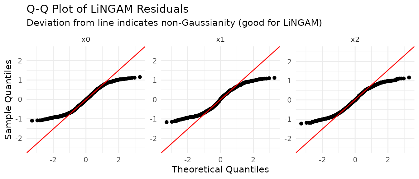

総因果効果

estimate_varma_total_effect() は、ある変数から別の変数への総因果効果を推定する。estimate_var_total_effect() のVARMA-LiNGAM版にあたり、psi（AR側）に加えて omega（MA側）の構造も積算する。VAR-LiNGAMと同様に、from_lag = 0（デフォルト）は同時点の総効果を、from_lag = 1 は $x_j(t-1)$ から $x_i(t)$ への1期先の効果を与える。

# Total effect x0 -> x2 (contemporaneous)
estimate_varma_total_effect(s_varma$data, model_varma, from_index = 1, to_index = 3)
#> [1] -0.2512211

# Total effect x0(t-1) -> x2(t) (one-step-ahead)
estimate_varma_total_effect(s_varma$data, model_varma, from_index = 1, to_index = 3, from_lag = 1)
#> [1] -0.1064222

ブートストラップ

lingam_varma_bootstrap()、get_varma_probabilities()、get_varma_paths() は VAR-LiNGAM版と対応しており、残差ブートストラップサンプルに対してVARMA-LiNGAMを再実行する。確率行列では、最初の 1 + p 個の列ブロックがpsi（ラグ）行列に、最後の q 個のブロックがomega（MA）行列に対応する。

bs_varma <- lingam_varma_bootstrap(
  s_varma$data,
  n_sampling = 100L,
  order      = c(1, 1),
  criterion  = NULL,
  seed       = 42,
  verbose    = FALSE
)
round(get_varma_probabilities(bs_varma, min_causal_effect = 0.1), 2)
#>      [,1] [,2] [,3] [,4] [,5] [,6] [,7] [,8] [,9]
#> [1,] 0.00    0    0 0.99 0.00 0.93 0.73 0.00 0.00
#> [2,] 1.00    0    0 0.75 1.00 0.84 0.09 0.01 0.06
#> [3,] 0.07    1    0 0.16 0.08 0.89 0.11 0.00 0.99

VARとVARMAのどちらを使うか

まずVAR-LiNGAMから始める。よりシンプルで高速であり、ラグ次数を情報量規準で自動選択できる。
ラグ次数を増やしてもVAR残差に自己相関が残る場合はVARMA-LiNGAMに切り替える。これは、有限次数のVARでは多数のラグでしか近似できないMA成分を撹乱項が持つ兆候である。
どちらの手法も定常性を仮定する。check_var_stationarity() / check_varma_stationarity() で確認し、単位根が疑われる場合は系列を差分する。

手法選択ガイド — データに合う手法の選び方
Direct LiNGAM 詳説 — i.i.d.向けの基本手法
ブートストラップと診断 — 推定構造の信頼性評価

VAR-LiNGAM：時系列データの因果探索

サンプルデータ

VAR-LiNGAMのあてはめ

ラグ次数の選択

定常性の確認

残差診断

総因果効果

ブートストラップ

VARMA-LiNGAM：移動平均誤差を持つ時系列

残差診断

総因果効果

ブートストラップ

VARとVARMAのどちらを使うか

関連記事