
この記事は、i.i.d.の連続データに対する lingamr
の中核推定器である lingam_direct()
の詳説である。出力の読み方、総因果効果の推定、事前知識の
組み込み、回帰手法の選択、そして失敗するケースとその理由を扱う。パッケージの
最初の一巡りには vignette("lingamr-ja")
を、データに合う手法の選び方には 手法選択ガイドを参照。
サンプルデータ
lingamr
は5種類の汎用サンプルデータ生成関数を提供する(他の推定器向けには
手法別の生成関数が別途ある)。いずれも
data(データフレーム) と
true_adjacency(真の隣接行列)を含むリストを返す。
| 関数 | 変数数 | デフォルトn | 特徴 |
|---|---|---|---|
generate_lingam_sample_6() |
6 | 1,000 | 標準的な固定構造。本記事の主な例 |
generate_lingam_sample_10() |
10 | 1,000 | 6変数ケースの拡張版(より大きなデータセット(10変数) で使用) |
generate_lingam_hard_sample() |
9 | 200 | 強い多重共線性を持つ難しい設定(強い多重共線性 で使用) |
generate_lingam_large_sample() |
可変 | 1,000 | 任意の変数数を持つランダムなスパースDAG(変数が多い場合:スケーラビリティの壁 で使用) |
generate_lingam_paradox_data() |
4 | 2,000 | 測定誤差パラドックス(パラドックスの例 で使用) |
generate_lingam_sample_6()
generate_lingam_sample_6()
は、6変数のLiNGAMモデルに従う人工データを、真の隣接行列
とともに返す。データは data に、隣接行列は
true_adjacency に格納される。
x1k <- generate_lingam_sample_6(n = 1000)

x1k$data |>
  head()
#>         x0        x1       x2        x3        x4        x5
#> 1 2.814924 18.017120 4.543655 0.6333728 18.160090 12.236660
#> 2 1.889685 10.956005 2.188091 0.3175366 13.172754  7.932657
#> 3 1.008905  6.990652 1.953131 0.2409218  6.702107  4.797122
#> 4 1.965690 12.296763 2.847148 0.3784141 13.224002  8.685252
#> 5 1.698178  9.698147 2.145058 0.3521443 11.673495  7.366258
#> 6 1.412372  8.640107 1.929980 0.2977585 10.024075  6.340899
x1k$true_adjacency
#>    x0 x1 x2 x3 x4 x5
#> x0  0  0  0  3  0  0
#> x1  3  0  2  0  0  0
#> x2  0  0  0  6  0  0
#> x3  0  0  0  0  0  0
#> x4  8  0 -1  0  0  0
#> x5  4  0  0  0  0  0
plot_adjacency()
は隣接行列に基づいて因果グラフを描画する。
x1k$true_adjacency |>
  plot_adjacency(
    labels  = colnames(x1k$data),
    title   = "True causal structure",
    rankdir = "TB",
    shape   = "circle"
  )
因果探索
lingam_direct() はDirect
LiNGAMを実行する。デフォルトでは、独立性の評価に相互情報量
が用いられ、パス係数はadaptive LASSO回帰で計算される。
model <- x1k$data |>
lingam_direct()独立性の評価にHSICを使うには、measure 引数を “kernel”
に設定する。HSICは計算コスト が高いため、n > 1000 では
lingam_direct() は自動的に低ランク近似に切り替わる。
因果順序
推定された因果順序は、インデックス番号として
causal_order に格納される。
# index number
model$causal_order
#> [1] 4 3 1 5 6 2

# variable name
colnames(x1k$data)[model$causal_order]
#> [1] "x3" "x2" "x0" "x4" "x5" "x1"
推定された隣接行列
推定された効果の大きさを確認する。デフォルトでは、adaptive LASSO回帰による回帰係数 が使われる。
model$adjacency_matrix |>
  round(3)
#>       x0 x1     x2    x3 x4 x5
#> x0 0.000  0  0.000 3.033  0  0
#> x1 2.988  0  2.002 0.000  0  0
#> x2 0.000  0  0.000 5.993  0  0
#> x3 0.000  0  0.000 0.000  0  0
#> x4 8.000  0 -1.000 0.000  0  0
#> x5 4.015  0  0.000 0.000  0  0
因果グラフの描画
Direct LiNGAMで推定した隣接行列に基づいて因果グラフを描画する。
model$adjacency_matrix |>
  plot_adjacency(
    labels    = colnames(model$adjacency_matrix),
    title     = "Estimated Causal Structure (Direct LiNGAM)",
    rankdir   = "TB",
    shape     = "ellipse",
    fillcolor = "lightgreen"
  )
推定構造と真の構造の比較
サンプルデータのように真の構造が既知の場合、plot_adjacency()
の true_B 引数に
真の隣接行列を渡すことで、推定されたエッジを真の構造と比較して色分けできる。これに
より推定精度を一目で評価でき、手法の検証や教育目的に有用である。
- 緑(実線): 正しく検出されたエッジ(推定・真とも存在)
- 赤(実線): 誤って検出されたエッジ(推定にはあるが真にはない)
- オレンジ(破線): 見逃されたエッジ(真にはあるが推定されなかった。真の係数を表示)
model$adjacency_matrix |>
  plot_adjacency(
    labels  = colnames(model$adjacency_matrix),
    true_B  = x1k$true_adjacency,
    title   = "Estimated vs. True Structure",
    rankdir = "TB",
    shape   = "ellipse"
  )
ggplot2による静的プロット
plot_adjacency()
はDiagrammeRによるインタラクティブなHTML図を返すのに対し、
autoplot()
は同じ因果構造をggplot2ベースの静的な図として描画する。これはR Markdown
/ Quartoでの画像・PDF出力で安定しており、後からggplot2の関数を重ねて
テーマやタイトルを設定することもできる。ノードの配置は
igraph の階層レイアウトで
計算されるため、因果の流れはおおむね上から下へと向かう。
autoplot()
はggplot2のジェネリック関数なので、ggplot2::autoplot()
として呼ぶか、 あらかじめ library(ggplot2)
で読み込んでおく(プロットには ggplot2 と
igraph が必要)。
ggplot2::autoplot(model)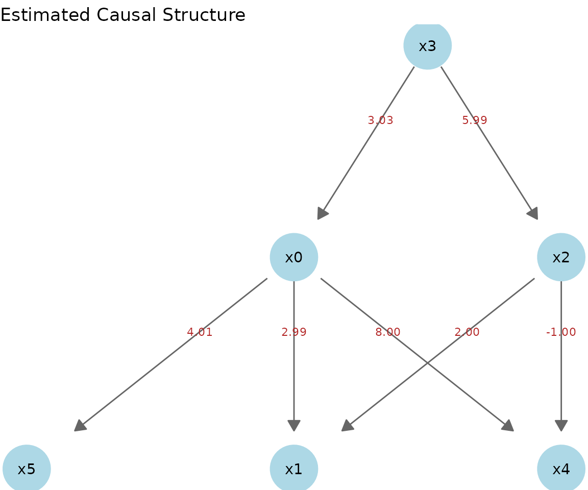
総因果効果
総因果効果とは、ある変数を1単位変化させたときの全体的な影響であり、直接効果と すべての間接効果(媒介変数を経由するパス)を合わせたものを指す。
total_effects <- x1k$data |>
  estimate_all_total_effects(model)

round(total_effects, 3)
#>       x0 x1     x2     x3 x4 x5
#> x0 0.000  0  0.000  3.033  0  0
#> x1 2.872  0  1.937 21.059  0  0
#> x2 0.000  0  0.000  5.993  0  0
#> x3 0.000  0  0.000  0.000  0  0
#> x4 7.910  0 -1.129 18.276  0  0
#> x5 4.015  0  0.000 12.179  0  0
重回帰係数との比較
媒介変数が存在する場合、重回帰係数と総因果効果は一致しない。
generate_lingam_sample_6()
の真の因果構造では、x3からx1へのパスが2つ存在する
(x3からx1への直接エッジは存在しない)。
- x3 -> x0 -> x1(間接効果: 3.0 x 3.0 = 9.0)
- x3 -> x2 -> x1(間接効果: 6.0 x 2.0 = 12.0)
- x3のx1への総因果効果 = 9.0 + 12.0 = 21.0
x1を予測するためにすべての変数を含むOLS回帰の係数を、estimate_all_total_effects()
の結果と比較する。
# Multiple regression: include all variables to predict x1
lm_coefs <- coef(lm(x1 ~ ., data = x1k$data))

# Comparison (variables causally related to x1: x0, x2, x3)
data.frame(
  variable           = c("x0", "x2", "x3"),
  OLS_coefficient    = round(lm_coefs[c("x0", "x2", "x3")], 3),
  total_causal_effect = round(total_effects["x1", c("x0", "x2", "x3")], 3)
)
#>    variable OLS_coefficient total_causal_effect
#> x0       x0           3.237               2.872
#> x2       x2           1.965               1.937
#> x3 x3 0.014 21.059x3のOLS係数はほぼ0である。これは、媒介変数であるx0とx2をモデルに含めることで、 x3の「媒介を通じた効果」がx0とx2の係数に吸収されてしまうためである。
一方、estimate_all_total_effects()
によるx3の値は約21であり、x3を1単位動かした
ときにx1が最終的にどれだけ変化するかを正しく表している。
| 問い | 使うべき指標 |
|---|---|
| 「x0とx2を固定したまま、x3を動かすとx1はどう変化するか」 | OLS重回帰係数 |
| 「すべてのパスを通じて、x3を動かすとx1はどう変化するか」 | 総因果効果 |
「ある変数に介入したときの最終的な影響」を知りたい場合は、重回帰係数ではなく総因果 効果を使う。
特定の変数ペア間の効果
estimate_all_total_effects()は全ペアの効果を一度に行列として返す。特定の
from -> toの1組だけが必要な場合は、estimate_total_effect()で直接計算
できる。from_index・to_indexは変数名・1始まりのインデックスのどちらでも
指定できる。
te_x3_x1 <- x1k$data |>
  estimate_total_effect(model, from_index = "x3", to_index = "x1")

round(te_x3_x1, 3)
#>     x3
#> 21.059

# Same value as the x3 column of the total_effects matrix computed above
isTRUE(all.equal(te_x3_x1, total_effects["x1", "x3"], check.attributes = FALSE))
#> [1] TRUE
事前知識を用いた推定
make_prior_knowledge()
を使うと、変数間の因果関係に関するドメイン知識をDirect
LiNGAMに組み込むことができる。これにより探索空間が狭まり、推定が安定化する。
事前知識行列の形式
make_prior_knowledge() は
の整数行列を返す。行 = 結果変数(to)、 列 =
原因変数(from)というインデックス規約は、隣接行列と同じである。
| 値 | 意味 |
|---|---|
-1 |
不明(デフォルト。Direct LiNGAMが自由に探索する) |
0 |
このエッジは存在しない |
1 |
このエッジは確実に存在する |
以下は、各引数が行列にどう反映されるかを示す。
| 引数 | 設定される値 | 意味 |
|---|---|---|
exogenous_variables |
指定した変数の行全体 -> 0
|
どの変数からも影響を受けない(root変数) |
sink_variables |
指定した変数の列全体 -> 0
|
どの変数にも影響を及ぼさない(sink変数) |
paths |
pk[to, from] = 1 |
このエッジが存在することを指定 |
no_paths |
pk[to, from] = 0 |
このエッジが存在しないことを指定 |
変数は1始まりのインデックス、または(labels
引数を渡せば)変数名で指定 できる。
使用例
generate_lingam_sample_6()
の真の構造に関するドメイン知識を与える。
- x3(インデックス4)は外生変数であり、他のどの変数からも影響を受けない
- x1, x4, x5(インデックス2, 5, 6)はsink変数であり、他の変数に影響を及ぼさない
- x0とx2の間にはパスが存在しない(どちら向きにも)
インデックスによる指定
pk1 <- make_prior_knowledge(
  n_variables         = 6,
  exogenous_variables = 4,          # x3
  sink_variables      = c(2, 5, 6), # x1, x4, x5
  no_paths            = list(c(3, 1), c(1, 3)) # no x2<->x0
)

pk1
#>      [,1] [,2] [,3] [,4] [,5] [,6]
#> [1,]   -1    0    0   -1    0    0
#> [2,]   -1   -1   -1   -1    0    0
#> [3,]    0    0   -1   -1    0    0
#> [4,]    0    0    0   -1    0    0
#> [5,]   -1    0   -1   -1   -1    0
#> [6,]   -1    0   -1   -1    0   -1
行列の読み方: pk1["x1", "x3"] が -1
なら「x3->x1は不明(LiNGAMが探索する)」、 0
なら「x3->x1は存在しない」ことを意味する。
事前知識を用いたDirect LiNGAMの実行
prior_knowledge 引数に渡すだけで、探索に反映される。
model_pk1 <- x1k$data |>
  lingam_direct(prior_knowledge = pk1, lambda = "BIC")

cat("Causal Order: ", colnames(x1k$data)[model_pk1$causal_order], "\n")
#> Causal Order:  x3 x2 x0 x4 x5 x1
model_pk1$adjacency_matrix |>
  round(3)
#>       x0 x1     x2    x3 x4 x5
#> x0 0.000  0  0.000 3.033  0  0
#> x1 2.988  0  2.002 0.000  0  0
#> x2 0.000  0  0.000 5.993  0  0
#> x3 0.000  0  0.000 0.000  0  0
#> x4 8.000  0 -1.000 0.000  0  0
#> x5 4.015  0  0.000 0.000  0  0

model_pk1$adjacency_matrix |>
  plot_adjacency(
    labels    = colnames(model_pk1$adjacency_matrix),
    title     = "Estimated (with Prior Knowledge)",
    rankdir   = "TB",
    shape     = "circle",
    fillcolor = "lightgreen"
  )
回帰手法の選択(reg_method)
Direct
LiNGAMでは、因果順序が決定された後に回帰によって隣接行列が推定される。
reg_method 引数はその回帰手法を選択する。
reg_method |
glmnet |
スパース化 | 特徴 |
|---|---|---|---|
"ols" |
不要 | なし | すべてのエッジを推定する。健全性チェックやパッケージのない環境向け |
"lasso" |
必要 | あり | 弱いエッジを0に縮小する |
"adaptive_lasso" |
必要 | あり(強力) | デフォルト。真に0であるエッジを確実に0にできるoracle性を持つ |
"ridge" |
必要 | なし | 正則化で係数を安定化させる。多重共線性に頑健。スパース化はしない |
oracle性とは「サンプルサイズが増えるにつれて真の構造を確実に復元できる」という
理論的保証であり、通常は "adaptive_lasso"
が推奨される。
4手法の比較
fit_ols    <- lingam_direct(x1k$data, reg_method = "ols")
fit_lasso  <- lingam_direct(x1k$data, reg_method = "lasso",          lambda = "BIC")
fit_alasso <- lingam_direct(x1k$data, reg_method = "adaptive_lasso", lambda = "BIC")
fit_ridge  <- lingam_direct(x1k$data, reg_method = "ridge",          lambda = "BIC")

# Compare the adjacency matrices side by side
round(fit_ols$adjacency_matrix,    3)
#>       x0 x1     x2     x3     x4    x5
#> x0 0.000  0 -0.040  3.274  0.000 0.000
#> x1 3.237  0  1.965  0.014 -0.034 0.006
#> x2 0.000  0  0.000  5.993  0.000 0.000
#> x3 0.000  0  0.000  0.000  0.000 0.000
#> x4 7.992  0 -1.062  0.394  0.000 0.000
#> x5 3.873  0  0.069 -0.315  0.018 0.000
round(fit_lasso$adjacency_matrix,  3)
#>       x0 x1     x2    x3 x4 x5
#> x0 0.000  0  0.000 3.030  0  0
#> x1 2.939  0  1.965 0.185  0  0
#> x2 0.000  0  0.000 5.993  0  0
#> x3 0.000  0  0.000 0.000  0  0
#> x4 7.924  0 -0.960 0.000  0  0
#> x5 3.975  0  0.000 0.000  0  0
round(fit_alasso$adjacency_matrix, 3)
#>       x0 x1     x2    x3 x4 x5
#> x0 0.000  0  0.000 3.033  0  0
#> x1 2.988  0  2.002 0.000  0  0
#> x2 0.000  0  0.000 5.993  0  0
#> x3 0.000  0  0.000 0.000  0  0
#> x4 8.000  0 -1.000 0.000  0  0
#> x5 4.015  0  0.000 0.000  0  0
round(fit_ridge$adjacency_matrix,  3)
#>       x0 x1     x2     x3    x4    x5
#> x0 0.000  0 -0.017  3.132 0.000 0.000
#> x1 1.863  0  1.987  0.656 0.071 0.127
#> x2 0.000  0  0.000  5.993 0.000 0.000
#> x3 0.000  0  0.000  0.000 0.000 0.000
#> x4 7.927  0 -0.997  0.203 0.000 0.000
#> x5 2.407  0  0.254 -0.251 0.197 0.000
OLSとRidgeはすべてのエッジに非ゼロの係数を残す傾向があるのに対し、LASSOとAdaptive LASSOは余分なエッジを0に縮小する。Ridgeは係数の大きさを小さくするが、ゼロには しない。
lambdaの選択(LASSO / Adaptive LASSO共通)
罰則の強さ の選択は、推定のスパース性を直接左右する。
lambda |
方式 | スパース性 | 用途 |
|---|---|---|---|
"BIC" |
情報量規準 | 最も高い | デフォルト。小サンプルでも安定 |
"AIC" |
情報量規準 | 高い | BICよりやや多くのエッジが残る |
"lambda.min" |
CV(予測誤差最小) | 低い | 予測精度を優先。エッジが多くなる |
"lambda.1se" |
CV(1SEルール) | 中〜高 | CVの頑健なバリエーション |
"oracle" |
解析式(adaptive_lassoのみ) | - | 。理論的なoracle性を保証 |
# Compare BIC (default, sparsest) and lambda.min (minimum prediction error)
fit_bic     <- lingam_direct(x1k$data, lambda = "BIC")
fit_lam_min <- lingam_direct(x1k$data, lambda = "lambda.min")

# Number of nonzero edges
sum(fit_bic$adjacency_matrix     != 0)
#> [1] 7
sum(fit_lam_min$adjacency_matrix != 0)
#> [1] 7
強い多重共線性(init_method)
generate_lingam_hard_sample()
は、x0からx4までの5つのroot変数が1つの
強い共通因子を共有する(collinearity引数で強さを指定。デフォルト0.95)
データを生成する。どの変数も互いを引き起こしていないにもかかわらず、互いに
強く相関する。下流の4変数x5からx8は、これらのrootの線形結合として生成
される(x8はさらにx5・x6にも依存する)。これは、単一の目的変数の予測
変数間に生じる通常の多重共線性より難しい設定である。ここでは、ほぼ共線な
変数群が外生変数(root)自体であり、「rootの誤差項は互いに独立である」という
DirectLiNGAMの前提そのものが破られている。
hard <- generate_lingam_hard_sample()

head(hard$data)
#>          x0        x1        x2        x3        x4       x5       x6       x7
#> 1 1.0228248 0.8886297 0.9693088 0.9349473 0.7947395 5.298107 4.166792 4.281243
#> 2 0.4830486 0.4748335 0.2787734 0.2895976 0.2664368 2.228899 1.343471 2.033147
#> 3 0.3727160 0.3013776 0.4418671 0.3585968 0.4657222 2.435443 1.570280 1.732436
#> 4 1.1951289 1.1560823 1.1158846 1.0539815 1.0437446 6.023135 4.747024 5.105043
#> 5 0.4059819 0.3034858 0.2156491 0.3155540 0.2783906 1.961220 1.356371 1.488881
#> 6 0.9547901 0.9622644 0.8374879 0.8856775 0.9972516 4.823226 3.801561 3.977539
#>          x8
#> 1 10.173626
#> 2  4.010030
#> 3  4.205728
#> 4 11.537226
#> 5  3.830753
#> 6  8.669491
hard$true_adjacency
#>     x0  x1  x2 x3 x4 x5 x6 x7 x8
#> x0 0.0 0.0 0.0  0  0  0  0  0  0
#> x1 0.0 0.0 0.0  0  0  0  0  0  0
#> x2 0.0 0.0 0.0  0  0  0  0  0  0
#> x3 0.0 0.0 0.0  0  0  0  0  0  0
#> x4 0.0 0.0 0.0  0  0  0  0  0  0
#> x5 1.5 1.5 1.5  0  0  0  0  0  0
#> x6 0.0 1.0 1.0  1  1  0  0  0  0
#> x7 2.0 0.0 0.0  2  0  0  0  0  0
#> x8 0.0 0.0 0.0  0  0  1  1  0  0

# x0-x4 share a common factor and are therefore highly correlated
round(cor(hard$data[c("x0", "x1", "x2", "x3", "x4")]), 3)
#>       x0    x1    x2    x3    x4
#> x0 1.000 0.896 0.904 0.907 0.917
#> x1 0.896 1.000 0.918 0.907 0.908
#> x2 0.904 0.918 1.000 0.905 0.906
#> x3 0.907 0.907 0.905 1.000 0.904
#> x4 0.917 0.908 0.906 0.904 1.000
デフォルト設定でDirect LiNGAMを実行する。
fit_hard <- lingam_direct(hard$data)

colnames(hard$data)[fit_hard$causal_order]
#> [1] "x3" "x8" "x6" "x2" "x0" "x1" "x4" "x5" "x7"x0からx4が互いに依存しているため、推定された因果順序は真の構造を完全には
満たさない。これを直接確認する:
すべての真のエッジfrom -> toについて、
推定順序でfromがtoより前に来ているべきである。
true_edges <- which(hard$true_adjacency != 0, arr.ind = TRUE)
order_pos  <- match(seq_len(ncol(hard$data)), fit_hard$causal_order)

edge_check <- data.frame(
  from            = colnames(hard$data)[true_edges[, "col"]],
  to              = colnames(hard$data)[true_edges[, "row"]],
  order_respected = order_pos[true_edges[, "col"]] < order_pos[true_edges[, "row"]]
)

edge_check
#>    from to order_respected
#> 1    x0 x5            TRUE
#> 2    x0 x7            TRUE
#> 3    x1 x5            TRUE
#> 4    x1 x6           FALSE
#> 5    x2 x5            TRUE
#> 6    x2 x6           FALSE
#> 7    x3 x6            TRUE
#> 8    x3 x7            TRUE
#> 9    x4 x6           FALSE
#> 10   x5 x8           FALSE
#> 11   x6 x8           FALSE
sum(edge_check$order_respected)   # number of true edges correctly ordered
#> [1] 6
11本の真のエッジのうち、正しく順序付けられているのは6本のみである。残り
(すべてx6またはx8へのエッジ)は、真の親が推定順序で遅く配置されたために、
見逃されるか逆方向に推定されている。これはまさにgenerate_lingam_hard_sample()
が示そうとしている失敗モードである:
外生変数どうしが相関していると、回帰が
始まる前の因果順序探索の段階ですでに破綻しうる。
それでもx0 -> x7のエッジはたまたま正しく順序付けられており、これを使えば
init_methodが回帰段階だけに与える影響を切り分けて見ることができる。
estimate_total_effect()はデフォルトでAdaptive
LASSOの初期重みをOLSで推定する
(init_method = "ols")。init_method = "ridge"に切り替えると、交差検証付き
Ridge回帰を使うようになり、多重共線性の下でも安定する。
set.seed(0)
te_hard_ols <- hard$data |>
  estimate_total_effect(fit_hard, from_index = "x0", to_index = "x7", init_method = "ols")

te_hard_ridge <- hard$data |>
  estimate_total_effect(fit_hard, from_index = "x0", to_index = "x7", init_method = "ridge")

round(c(ols = unname(te_hard_ols), ridge = unname(te_hard_ridge)), 3)
#>   ols ridge
#> 3.624 2.590
x0 -> x7の真の係数は2.0である。OLS初期化の推定値は大きく超過するのに
対し、Ridge初期化の推定値は真の値にずっと近い – これはまさに
generate_lingam_hard_sample()のドキュメントが「強い多重共線性の下では
Ridge初期化Adaptive LASSOが望ましい」とする理由と一致する。ただし
init_methodが影響するのはこの回帰段階のみであり、因果順序探索は変えない。
したがって、上で示した順序の問題自体を解決するものではない。
非ガウス性の仮定
LiNGAMの理論的な核心は、誤差項が非ガウス分布に従うという仮定である。誤差が ガウス分布に従う場合、因果の方向は原理的に識別不能になり(同じ分布を説明する 逆方向のモデルが存在する)、推定結果は信頼できなくなる。
generate_lingam_sample_6() の noise_dist
引数で誤差分布を切り替え、この違いを
実際に確認する。真の構造は以下の通りである(rootはx3)。
set.seed(0)
truth <- generate_lingam_sample_6(noise_dist = "uniform")

truth$true_adjacency |>
  round(1)
#>    x0 x1 x2 x3 x4 x5
#> x0  0  0  0  3  0  0
#> x1  3  0  2  0  0  0
#> x2  0  0  0  6  0  0
#> x3  0  0  0  0  0  0
#> x4  8  0 -1  0  0  0
#> x5  4  0  0  0  0  0
真の構造の因果グラフ:
truth$true_adjacency |>
  plot_adjacency(
    labels = colnames(truth$data),
    title  = "True structure"
  )
非ガウス誤差(一様分布)でうまくいく場合
fit_uniform <- lingam_direct(truth$data)

# Estimated causal order (the true root x3 comes first)
colnames(truth$data)[fit_uniform$causal_order]
#> [1] "x3" "x2" "x0" "x4" "x5" "x1"

# The estimated adjacency matrix recovers the true structure almost perfectly
fit_uniform$adjacency_matrix |>
  round(1)
#>    x0 x1 x2 x3 x4 x5
#> x0  0  0  0  3  0  0
#> x1  3  0  2  0  0  0
#> x2  0  0  0  6  0  0
#> x3  0  0  0  0  0  0
#> x4  8  0 -1  0  0  0
#> x5  4  0  0  0  0  0
推定されたグラフは真の構造とほぼ一致する。エッジは真の構造と比較して色分けされる。 緑 = 正解、赤 = 誤検出、オレンジ破線 = 見逃し。
fit_uniform$adjacency_matrix |>
  plot_adjacency(
    labels = colnames(truth$data),
    true_B = truth$true_adjacency,
    title  = "Estimated (uniform errors)"
  )
ガウス誤差でうまくいかない場合
同じ因果構造でも、誤差がガウス分布に従うと結果は破綻する。
gauss <- generate_lingam_sample_6(noise_dist = "gaussian")
fit_gauss <- lingam_direct(gauss$data)

# The causal order does not match the true structure (root x3 does not come first)
colnames(gauss$data)[fit_gauss$causal_order]
#> [1] "x1" "x2" "x5" "x3" "x4" "x0"

fit_gauss$adjacency_matrix |>
  round(1)
#>    x0  x1   x2 x3  x4  x5
#> x0  0 0.1  0.0  0 0.1 0.0
#> x1  0 0.0  0.0  0 0.0 0.0
#> x2  0 0.3  0.0  0 0.0 0.0
#> x3  0 0.0  0.2  0 0.0 0.0
#> x4  0 0.9 -2.6  0 0.0 1.3
#> x5  0 1.2 -2.1  0 0.0 0.0
真の構造と比較すると、多くのエッジが誤り(赤)または見逃し(オレンジ破線)に なっている。色分けは上記と同じである。
fit_gauss$adjacency_matrix |>
  plot_adjacency(
    labels = colnames(gauss$data),
    true_B = truth$true_adjacency,
    title  = "Estimated (Gaussian errors)"
  )
非ガウス誤差では真の隣接行列がそのまま復元されるのに対し、ガウス誤差では因果順序と 係数の両方が真の構造から大きく乖離する。これが「LiNGAMはデータの非ガウス性を利用 して因果の方向を決定する」と言われる理由である。実データに適用する際は、残差の 正規性を検定し、この仮定が成り立っているかを確認することが重要である – ブートストラップと診断の記事を参照。
より大きなデータセット(10変数)
10変数・10,000行という、より大きなデータセットの例を示す。
x10k <- generate_lingam_sample_10(n = 10000)

x10k$true_adjacency |>
  plot_adjacency(
    labels  = colnames(x10k$data),
    title   = "True causal structure",
    rankdir = "TB",
    shape   = "circle"
  )
ICA-LiNGAMとDirect LiNGAMの比較
pcalg::lingam()
はオリジナルのLiNGAMアルゴリズムであり、FastICAで混合行列を推定
することで因果順序と係数を求める(Shimizu et
al. 2006)。lingam_direct() とは
独立したアプローチで同じ問題を解く。
両アルゴリズムの実行
同じ6変数データセット()を両手法で分析する。
d_cmp <- generate_lingam_sample_6(n = 1000, seed = 42)

t_cmp_direct <- system.time(res_cmp_direct <- lingam_direct(d_cmp$data))
t_cmp_ica    <- system.time(res_cmp_ica    <- pcalg::lingam(as.matrix(d_cmp$data)))

cat(sprintf("Direct LiNGAM : %.2f sec\nICA-LiNGAM    : %.2f sec\n",
            t_cmp_direct["elapsed"], t_cmp_ica["elapsed"]))
#> Direct LiNGAM : 0.01 sec
#> ICA-LiNGAM    : 0.02 sec
推定係数の比較
$Bpruned
はlingamrの隣接行列と同じ規約(B[i, j] =
の係数)を使う。
B_ica <- res_cmp_ica$Bpruned
rownames(B_ica) <- colnames(B_ica) <- names(d_cmp$data)

idx_ica  <- which(abs(B_ica) > 0, arr.ind = TRUE)
tidy_ica <- data.frame(
  from  = colnames(B_ica)[idx_ica[, 2]],
  to    = rownames(B_ica)[idx_ica[, 1]],
  ica   = round(B_ica[idx_ica], 3)
)

tidy_dir <- tidy(res_cmp_direct)
tidy_dir <- data.frame(from = tidy_dir$from, to = tidy_dir$to,
                       direct = round(tidy_dir$estimate, 3))

merge(tidy_dir, tidy_ica, by = c("from", "to"), sort = TRUE)
#>   from to direct    ica
#> 1   x0 x1  2.988  3.245
#> 2   x0 x4  8.000  7.999
#> 3   x0 x5  4.015  3.876
#> 4   x2 x1  2.002  1.973
#> 5   x2 x4 -1.000 -1.060
#> 6   x3 x0  3.033  3.027
#> 7   x3 x2  5.993  6.101
DAG構造の比較
すべてのエッジについて完全外部結合(full outer join)を取り、構造を比較し、真のDAG との整合性を確認する。
B_true   <- d_cmp$true_adjacency
idx_true <- which(abs(B_true) > 0, arr.ind = TRUE)
true_key <- paste(colnames(B_true)[idx_true[, 2]],
                  rownames(B_true)[idx_true[, 1]], sep = "->")

cmp <- merge(tidy_dir, tidy_ica, by = c("from", "to"), all = TRUE, sort = TRUE)
cmp$truth <- paste(cmp$from, cmp$to, sep = "->") %in% true_key
cmp
#>   from to direct    ica truth
#> 1   x0 x1  2.988  3.245  TRUE
#> 2   x0 x4  8.000  7.999  TRUE
#> 3   x0 x5  4.015  3.876  TRUE
#> 4   x2 x1  2.002  1.973  TRUE
#> 5   x2 x4 -1.000 -1.060  TRUE
#> 6   x3 x0  3.033  3.027  TRUE
#> 7   x3 x2  5.993  6.101  TRUE
direct または ica 列が NA
の場合、その手法がそのエッジを検出しなかったことを
意味する。truth = TRUE
は真のDAGに存在するエッジであることを示す。
変数が多い場合:スケーラビリティの壁
Direct LiNGAMは各ステップで、残っているすべての変数ペアについて独立性検定を行う。 ステップ数は で、各ステップの検定回数は最大 であるため、独立性検定の 総回数はおおよそ
となり、計算コストはになる。 一方、ICA-LiNGAMが使うFastICAは(BLAS最適化により)なので、変数の数が 増えるほどその差は広がる。
generate_lingam_large_sample() は、変数数 p
を自由に設定できるランダムな スパースDAGデータを生成する。各変数
()は、
の中からランダムに最大 max_parents
個の親を持つ。因果順序は必ずインデックス順に
従うため、隣接行列は常に下三角行列になる。
データの生成
d20 <- generate_lingam_large_sample(p = 20, n = 1000, seed = 42)

dim(d20$data)                    # 1000 rows x 20 columns
#> [1] 1000   20
sum(d20$true_adjacency != 0)     # number of true edges (sparse DAG)
#> [1] 32
d20$true_causal_order            # 0, 1, ..., 19
#>  [1]  0  1  2  3  4  5  6  7  8  9 10 11 12 13 14 15 16 17 18 19
実行時間の比較
が1.5倍(10 -> 15)になると、独立性検定の回数は 倍に 増える。
d10 <- generate_lingam_large_sample(p = 10, n = 500, seed = 42)
d15 <- generate_lingam_large_sample(p = 15, n = 500, seed = 42)

t10 <- system.time({ r10 <- lingam_direct(d10$data) })
t15 <- system.time({ r15 <- lingam_direct(d15$data) })

cat(sprintf(
  "p = 10 : %.2f sec\np = 15 : %.2f sec\ntheoretical factor %.1fx vs. observed %.1fx\n",
  t10["elapsed"],
  t15["elapsed"],
  15^3 / 10^3,
  t15["elapsed"] / max(t10["elapsed"], 0.01)
))
#> p = 10 : 0.03 sec
#> p = 15 : 0.06 sec
#> theoretical factor 3.4x vs. observed 2.1x
同じデータでICA-LiNGAMも実行し、速度を直接比較する。
t10_ica <- system.time({ pcalg::lingam(as.matrix(d10$data)) })
t15_ica <- system.time({ pcalg::lingam(as.matrix(d15$data)) })

cat(sprintf(
  "              p = 10   p = 15\nDirect LiNGAM : %5.2f sec  %5.2f sec\nICA-LiNGAM    : %5.2f sec  %5.2f sec\n",
  t10["elapsed"], t15["elapsed"],
  t10_ica["elapsed"], t15_ica["elapsed"]
))
#>               p = 10   p = 15
#> Direct LiNGAM :  0.03 sec   0.06 sec
#> ICA-LiNGAM : 0.02 sec 0.03 secが大きくなるほどDirect LiNGAMのコストが支配的になり、両者の差は広がる。 やのような大規模な設定では、この傾向はさらに顕著になる。
推定精度の確認(p = 10)
スパースDAGであっても、非ガウス誤差(デフォルト: 一様分布)である限り、Direct LiNGAMは正しい因果順序を復元できる。
# Estimated causal order
r10$causal_order
#>  [1]  1  2  3  7  4  5  9  8  6 10

# Whether it matches the true causal order 0, 1, ..., 9 exactly
all(r10$causal_order == d10$true_causal_order)
#> [1] FALSE
tidy() でエッジリストに変換し、推定係数を確認する。
高次元Direct LiNGAM
上で示したの独立性検定コストは、が数十〜数百のオーダーになると実質的な ボトルネックとなり、(変数数が観測数を上回る)になると、通常の回帰ベースの 隣接行列推定がそもそも成立しなくなる。
lingam_high_dim()
は、この領域向けに設計されたHighDimDirectLiNGAM(Wang & Drton
2020)を実装したものである。ペアワイズの独立性検定の代わりに、キャッシュされた
グラム行列から計算される非ガウス性のモーメント統計量を用いて因果順序を探索する。
このアルゴリズムは決定的(ランダムな再試行なし)であり、lingam_direct()
と同じ LingamResult
オブジェクトを返すため、print()、tidy()、plot_adjacency()、
estimate_total_effect() はすべてそのまま使用できる。
hd_sample <- generate_lingam_sample_6(n = 500, seed = 1)
hd_result <- lingam_high_dim(hd_sample$data)

hd_result$causal_order
#> [1] 4 3 1 5 2 6
round(hd_result$adjacency_matrix, 3)
#>       x0 x1     x2    x3 x4 x5
#> x0 0.000  0  0.000 2.968  0  0
#> x1 2.970  0  2.013 0.000  0  0
#> x2 0.000  0  0.000 6.010  0  0
#> x3 0.000  0  0.000 0.000  0  0
#> x4 8.023  0 -1.000 0.000  0  0
#> x5 4.013  0  0.000 0.000  0  0
n_samples <= n_features
の場合、隣接行列の推定に通常のBICベースのAdaptive LASSOは
使えないため、lingam_high_dim()
は交差検証済みLASSO(glmnet::cv.glmnet)に
フォールバックし、警告を発する。
wide_sample <- generate_lingam_large_sample(p = 30, n = 25, seed = 1)
wide_result <- lingam_high_dim(wide_sample$data)
#> Warning: Since n_samples <= n_features, the adjacency matrix is estimated with
#> cross-validated lasso (cv.glmnet) instead of BIC-based lambda selection.
#> Warning: Option grouped=FALSE enforced in cv.glmnet, since < 3 observations per
#> fold
#> Warning: Option grouped=FALSE enforced in cv.glmnet, since < 3 observations per
#> fold
#> Warning: Option grouped=FALSE enforced in cv.glmnet, since < 3 observations per
#> fold
#> Warning: Option grouped=FALSE enforced in cv.glmnet, since < 3 observations per
#> fold
#> Warning: Option grouped=FALSE enforced in cv.glmnet, since < 3 observations per
#> fold
#> Warning: Option grouped=FALSE enforced in cv.glmnet, since < 3 observations per
#> fold
#> Warning: Option grouped=FALSE enforced in cv.glmnet, since < 3 observations per
#> fold
#> Warning: Option grouped=FALSE enforced in cv.glmnet, since < 3 observations per
#> fold
#> Warning: Option grouped=FALSE enforced in cv.glmnet, since < 3 observations per
#> fold
#> Warning: Option grouped=FALSE enforced in cv.glmnet, since < 3 observations per
#> fold
#> Warning: Option grouped=FALSE enforced in cv.glmnet, since < 3 observations per
#> fold
#> Warning: Option grouped=FALSE enforced in cv.glmnet, since < 3 observations per
#> fold
#> Warning: Option grouped=FALSE enforced in cv.glmnet, since < 3 observations per
#> fold
#> Warning: Option grouped=FALSE enforced in cv.glmnet, since < 3 observations per
#> fold
#> Warning: Option grouped=FALSE enforced in cv.glmnet, since < 3 observations per
#> fold
#> Warning: Option grouped=FALSE enforced in cv.glmnet, since < 3 observations per
#> fold
#> Warning: Option grouped=FALSE enforced in cv.glmnet, since < 3 observations per
#> fold
#> Warning: Option grouped=FALSE enforced in cv.glmnet, since < 3 observations per
#> fold
#> Warning: Option grouped=FALSE enforced in cv.glmnet, since < 3 observations per
#> fold
#> Warning: Option grouped=FALSE enforced in cv.glmnet, since < 3 observations per
#> fold
#> Warning: Option grouped=FALSE enforced in cv.glmnet, since < 3 observations per
#> fold
#> Warning: Option grouped=FALSE enforced in cv.glmnet, since < 3 observations per
#> fold
#> Warning: Option grouped=FALSE enforced in cv.glmnet, since < 3 observations per
#> fold
#> Warning: Option grouped=FALSE enforced in cv.glmnet, since < 3 observations per
#> fold
#> Warning: Option grouped=FALSE enforced in cv.glmnet, since < 3 observations per
#> fold
#> Warning: Option grouped=FALSE enforced in cv.glmnet, since < 3 observations per
#> fold
#> Warning: Option grouped=FALSE enforced in cv.glmnet, since < 3 observations per
#> fold
#> Warning: Option grouped=FALSE enforced in cv.glmnet, since < 3 observations per
#> fold

wide_result$causal_order
#>  [1]  2  1  3  8 20 13 27  4  5 12 26  6  7 16  9 15 14 23 10 18 21 11 22 24 29
#> [26] 30 25 19 17 28
DirectLiNGAMが苦手とする例:測定誤差パラドックス
因果探索の手法にはそれぞれ仮定があり、それが破られると正しい構造を復元できないこと
がある。generate_lingam_paradox_data()
は、意図的にそうした困難な状況を作り出す
ために設計されたデータセットである。他のサンプル生成関数と同様に、data
と true_adjacency を含むリストを返す。
このデータの真の構造は単純な直列連鎖 x0 -> x1 -> x2 -> x3(各係数0.8)である。 しかし、注目すべき特徴が2つある。
- root変数x0に大きな測定誤差が加えられている。 これにより、DirectLiNGAMの最初の ステップで行われる独立性評価が乱され、rootを誤って選んでしまい、誤差が伝播しやす くなる。
- すべての変数が
scale()で標準化されている(スケールの違いはない)。
paradox <- generate_lingam_paradox_data(n = 2000L, seed = 42)

head(paradox$data)
#>             x0         x1          x2         x3
#> 1  0.780627610  2.0872183  1.95046049  1.1209218
#> 2  0.529343129  1.1562639  1.86870201  1.6129261
#> 3 -1.193165251 -0.2515850 -0.43614264 -0.9056694
#> 4 -0.056001104  1.6615506  2.07542227  0.7890187
#> 5  0.004312424  1.0175487 -0.02532253 -0.3155891
#> 6  0.658064158  0.4833892  0.25385608  0.0167021

# All variables are standardized (sd = 1)
sapply(paradox$data, sd)
#> x0 x1 x2 x3
#>  1  1  1  1
真の因果グラフを可視化する。係数0.8は、標準化前の潜在スケールにおける構造係数である。
paradox$true_adjacency |>
  plot_adjacency(
    labels  = colnames(paradox$true_adjacency),
    title   = "True causal chain (x0 -> x1 -> x2 -> x3)",
    rankdir = "LR",
    shape   = "circle"
  )
ここでDirect LiNGAMを適用してみる。
model_p <- lingam_direct(paradox$data)

# Estimated causal order
colnames(paradox$data)[model_p$causal_order]
#> [1] "x1" "x2" "x0" "x3"推定された因果順序の先頭がx1であり、真のrootであるx0ではない点に注意する。 rootの測定誤差のせいで、DirectLiNGAMは最初の外生変数としてx0を選ぶことに失敗して いる。
model_p$adjacency_matrix |>
  round(3)
#>    x0    x1    x2 x3
#> x0  0 0.558 0.000  0
#> x1  0 0.000 0.000  0
#> x2  0 0.833 0.000  0
#> x3  0 0.000 0.822  0

model_p$adjacency_matrix |>
  plot_adjacency(
    labels    = colnames(model_p$adjacency_matrix),
    title     = "Estimated structure (paradox data)",
    rankdir   = "LR",
    shape     = "circle",
    fillcolor = "lightpink"
)下流のx1 -> x2 -> x3は正しく復元されているものの、x0とx1の間の方向は逆転 しており(真はx0 -> x1だが、推定はx1 -> x0)、x0はほとんどsinkのように扱われて しまっている。
このエラーが偶然生じたものか、それとも系統的なものかを、ブートストラップで確認する。
bs_paradox <- paradox$data |>
  lingam_direct_bootstrap(n_sampling = 100L, seed = 42)
#> Bootstrap: 100 iterations, method=adaptive_lasso (sequential)
#>   iteration 1 / 100
#>   iteration 10 / 100
#>   iteration 20 / 100
#>   iteration 30 / 100
#>   iteration 40 / 100
#>   iteration 50 / 100
#>   iteration 60 / 100
#>   iteration 70 / 100
#>   iteration 80 / 100
#>   iteration 90 / 100
#>   iteration 100 / 100
#> Completed in 1.5 seconds.

# Occurrence probability of each direction (row = to, column = from)
bs_paradox |>
  get_probabilities() |>
  round(2)
#>      [,1] [,2] [,3] [,4]
#> [1,]    0    1 0.05 0.01
#> [2,]    0    0 0.00 0.00
#> [3,]    0    1 0.00 0.00
#> [4,] 0 0 1.00 0.00重要なのは、誤った方向であるx1 -> x0がほぼ100%の確率で再現されている点である。 つまり、このエラーは偶然ではなく系統的であり、ブートストラップサンプル全体で 安定して現れる。
教訓: ブートストラップの安定性(高い再現確率)は、推定の正しさを保証する ものではない。モデルの仮定(ここでは「上流の変数に測定誤差がない」という仮定)が 破られている場合、その手法は安定して誤った構造を復元してしまうことがある。 残差の独立性・正規性の検定や、データ生成過程に関するドメイン知識と併せて、結果を 批判的に評価することが重要である。
関連記事
- 手法選択ガイド — データに合う手法の選び方
- ブートストラップと診断 — 信頼性の評価と仮定の確認
- 時系列(VAR-LiNGAMとVARMA-LiNGAM)
- 潜在交絡変数(ParceLiNGAMとRCD)
- 非線形の手法(RESITとCAM-UV)
- 特殊なデータ(LiM・MultiGroup・欠測値)