
This article is a deep dive into lingam_direct(), the
core estimator of lingamr for i.i.d. continuous data: how
to read its output, estimate total causal effects, incorporate prior
knowledge, choose the regression method, and understand when and why it
fails. For a first tour of the package, start with
vignette("lingamr"); to pick the right method for your
data, see the method selection
guide.
Sample Data
lingamr provides five general-purpose sample data
generators (further method-specific generators exist for the other
estimators). Each returns a list containing data (a data
frame) and true_adjacency (the true adjacency matrix).
| Function | Variables | Default n | Characteristics |
|---|---|---|---|
generate_lingam_sample_6() |
6 | 1,000 | Standard fixed structure. The main example in this article |
generate_lingam_sample_10() |
10 | 1,000 | An extension of the 6-variable case (used in A Larger Dataset) |
generate_lingam_hard_sample() |
9 | 200 | A difficult setting with strong multicollinearity (used in Strong Multicollinearity) |
generate_lingam_large_sample() |
variable | 1,000 | A random sparse DAG with an arbitrary number of variables (used in The Scalability Wall) |
generate_lingam_paradox_data() |
4 | 2,000 | The measurement error paradox (used in The Paradox Example) |
generate_lingam_sample_6()
generate_lingam_sample_6() returns artificial data
following a 6-variable LiNGAM model, together with its true adjacency
matrix. The data is stored in data and the adjacency matrix
in true_adjacency.
x1k <- generate_lingam_sample_6(n = 1000)

x1k$data |>
  head()
#>         x0        x1       x2        x3        x4        x5
#> 1 2.814924 18.017120 4.543655 0.6333728 18.160090 12.236660
#> 2 1.889685 10.956005 2.188091 0.3175366 13.172754  7.932657
#> 3 1.008905  6.990652 1.953131 0.2409218  6.702107  4.797122
#> 4 1.965690 12.296763 2.847148 0.3784141 13.224002  8.685252
#> 5 1.698178  9.698147 2.145058 0.3521443 11.673495  7.366258
#> 6 1.412372  8.640107 1.929980 0.2977585 10.024075  6.340899
x1k$true_adjacency
#>    x0 x1 x2 x3 x4 x5
#> x0  0  0  0  3  0  0
#> x1  3  0  2  0  0  0
#> x2  0  0  0  6  0  0
#> x3  0  0  0  0  0  0
#> x4  8  0 -1  0  0  0
#> x5  4  0  0  0  0  0
plot_adjacency() draws a causal graph based on the
adjacency matrix.
x1k$true_adjacency |>
  plot_adjacency(
    labels  = colnames(x1k$data),
    title   = "True causal structure",
    rankdir = "TB",
    shape   = "circle"
  )
Causal Discovery
lingam_direct() runs Direct LiNGAM. By default,
independence is assessed using mutual information, and path coefficients
are computed with adaptive LASSO regression.
model <- x1k$data |>
  lingam_direct()
To use HSIC for assessing independence, set the measure
argument to “kernel”. HSIC is computationally expensive; for
n > 1000, lingam_direct() automatically
switches to a low-rank approximation.
Causal Order
The estimated causal order is stored in causal_order as
index numbers.
# index number
model$causal_order
#> [1] 4 3 1 5 6 2

# variable name
colnames(x1k$data)[model$causal_order]
#> [1] "x3" "x2" "x0" "x4" "x5" "x1"
Estimated Adjacency Matrix
We inspect the estimated effect magnitudes. By default, the regression coefficients from adaptive LASSO regression are used.
model$adjacency_matrix |>
  round(3)
#>       x0 x1     x2    x3 x4 x5
#> x0 0.000  0  0.000 3.033  0  0
#> x1 2.988  0  2.002 0.000  0  0
#> x2 0.000  0  0.000 5.993  0  0
#> x3 0.000  0  0.000 0.000  0  0
#> x4 8.000  0 -1.000 0.000  0  0
#> x5 4.015  0  0.000 0.000  0  0
Drawing the Causal Graph
We draw the causal graph based on the adjacency matrix estimated by Direct LiNGAM.
model$adjacency_matrix |>
  plot_adjacency(
    labels    = colnames(model$adjacency_matrix),
    title     = "Estimated Causal Structure (Direct LiNGAM)",
    rankdir   = "TB",
    shape     = "ellipse",
    fillcolor = "lightgreen"
  )
Comparing the Estimated and True Structures
When the true structure is known, as with sample data, you can pass
the true adjacency matrix to the true_B argument of
plot_adjacency() to color-code the estimated edges by
comparing them against the true structure. This lets you assess
estimation accuracy at a glance, which is useful for validating methods
or for educational purposes.
- Green (solid): correctly detected edges (estimated and true)
- Red (solid): falsely detected edges (estimated but not true)
- Orange (dashed): missed edges (true but not estimated; the true coefficient is shown)
model$adjacency_matrix |>
  plot_adjacency(
    labels  = colnames(model$adjacency_matrix),
    true_B  = x1k$true_adjacency,
    title   = "Estimated vs. True Structure",
    rankdir = "TB",
    shape   = "ellipse"
  )
Static Plotting with ggplot2
While plot_adjacency() returns an interactive HTML
figure via DiagrammeR, autoplot() draws the same causal
structure as a static, ggplot2-based figure. This is stable for image
and PDF output in R Markdown / Quarto, and you can layer ggplot2
functions on top to set themes or titles afterward. Node positions are
computed using igraph’s hierarchical layout, so the causal
flow generally runs from top to bottom.
autoplot() is a ggplot2 generic, so call it as
ggplot2::autoplot() or load it beforehand with
library(ggplot2) (plotting requires ggplot2
and igraph).
ggplot2::autoplot(model)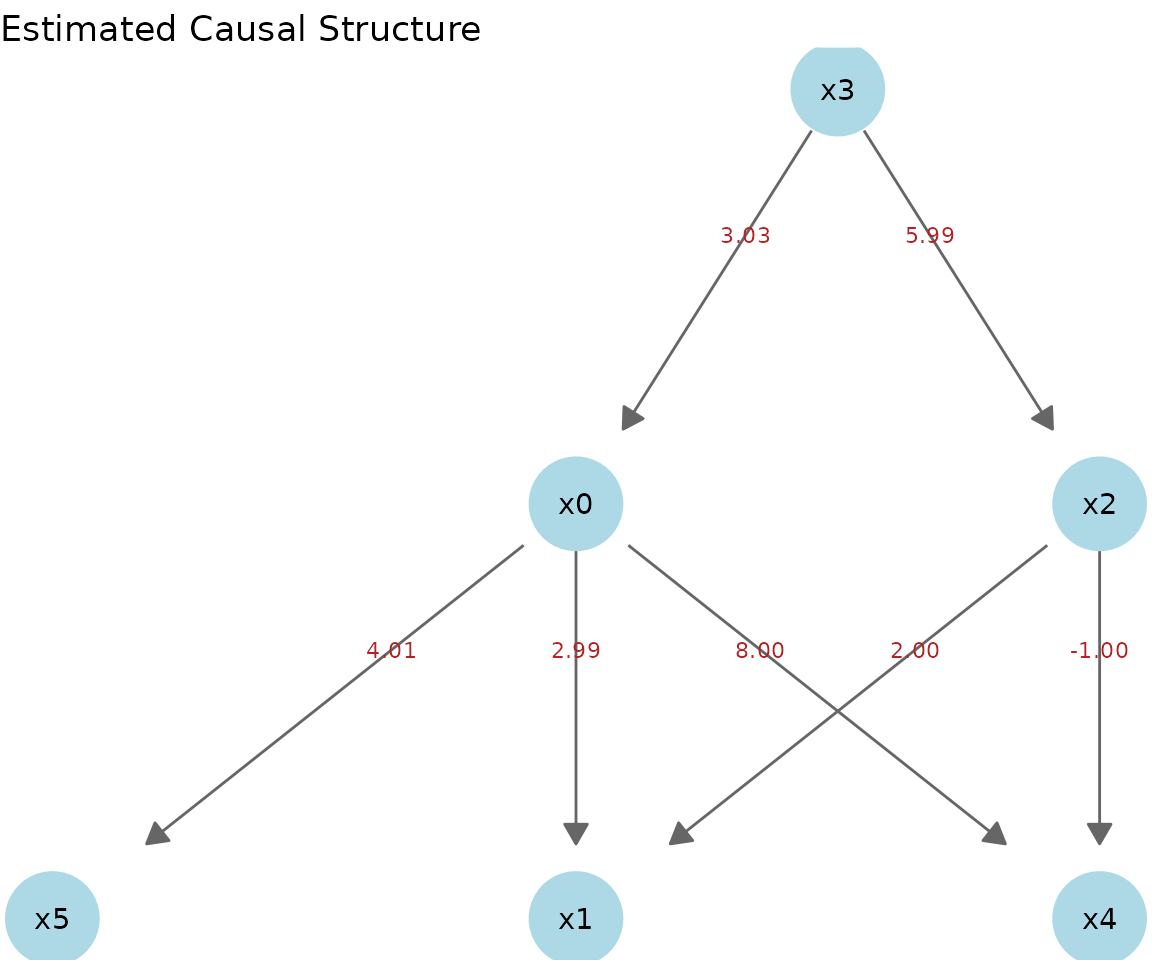
Total Causal Effect
The total causal effect is the overall impact of changing one variable by one unit, combining the direct path and all indirect paths (paths through mediating variables).
total_effects <- x1k$data |>
  estimate_all_total_effects(model)

round(total_effects, 3)
#>       x0 x1     x2     x3 x4 x5
#> x0 0.000  0  0.000  3.033  0  0
#> x1 2.872  0  1.937 21.059  0  0
#> x2 0.000  0  0.000  5.993  0  0
#> x3 0.000  0  0.000  0.000  0  0
#> x4 7.910  0 -1.129 18.276  0  0
#> x5 4.015  0  0.000 12.179  0  0
Comparison with Multiple Regression Coefficients
Multiple regression coefficients and total causal effects do not agree when mediating variables are present.
In the true causal structure of
generate_lingam_sample_6(), there are two paths from x3 to
x1 (there is no direct edge from x3 to x1).
- x3 -> x0 -> x1 (indirect effect: 3.0 x 3.0 = 9.0)
- x3 -> x2 -> x1 (indirect effect: 6.0 x 2.0 = 12.0)
- Total causal effect of x3 on x1 = 9.0 + 12.0 = 21.0
We compare the coefficients from an OLS regression that includes all
variables to predict x1 against the results of
estimate_all_total_effects().
# Multiple regression: include all variables to predict x1
lm_coefs <- coef(lm(x1 ~ ., data = x1k$data))

# Comparison (variables causally related to x1: x0, x2, x3)
data.frame(
  variable           = c("x0", "x2", "x3"),
  OLS_coefficient    = round(lm_coefs[c("x0", "x2", "x3")], 3),
  total_causal_effect = round(total_effects["x1", c("x0", "x2", "x3")], 3)
)
#>    variable OLS_coefficient total_causal_effect
#> x0       x0           3.237               2.872
#> x2       x2           1.965               1.937
#> x3       x3           0.014              21.059
The OLS coefficient for x3 is nearly 0. This is because including x0 and x2 (the mediating variables) in the model causes x3’s “effect through mediation” to be absorbed into the coefficients of x0 and x2.
In contrast, the value of x3 from
estimate_all_total_effects() is ~21, which
correctly represents how much x1 ultimately changes when x3 is moved by
one unit.
| Question | Metric to use |
|---|---|
| “How does x1 change if I move x3 while holding x0 and x2 fixed?” | OLS multiple regression coefficient |
| “How does x1 change if I move x3, through all paths?” | Total causal effect |
When you want to know “the ultimate impact of intervening on a variable,” use the total causal effect rather than the multiple regression coefficient.
Effect Between a Single Pair of Variables
estimate_all_total_effects() returns the full matrix of
pairwise effects at once. When only one specific
from -> to pair is needed,
estimate_total_effect() computes it directly;
from_index and to_index accept either a
variable name or a 1-based index.
te_x3_x1 <- x1k$data |>
  estimate_total_effect(model, from_index = "x3", to_index = "x1")

round(te_x3_x1, 3)
#>     x3
#> 21.059

# Same value as the x3 column of the total_effects matrix computed above
isTRUE(all.equal(te_x3_x1, total_effects["x1", "x3"], check.attributes = FALSE))
#> [1] TRUE
Inference with Prior Knowledge
With make_prior_knowledge(), you can incorporate domain
knowledge about the causal relationships among variables into Direct
LiNGAM. This narrows the search space and stabilizes estimation.
Format of the Prior Knowledge Matrix
make_prior_knowledge() returns a
integer matrix. It uses the indexing convention row = effect
variable (to), column = cause variable (from), the same
convention as the adjacency matrix.
| Value | Meaning |
|---|---|
-1 |
Unknown (default; Direct LiNGAM searches freely) |
0 |
This edge does not exist |
1 |
This edge definitely exists |
The following shows how each argument affects the matrix.
| Argument | Value set | Meaning |
|---|---|---|
exogenous_variables |
the entire row of the specified variable ->
0
|
Receives no influence from any variable (root variable) |
sink_variables |
the entire column of the specified variable ->
0
|
Exerts no influence on any variable (sink variable) |
paths |
pk[to, from] = 1 |
Specifies that this edge exists |
no_paths |
pk[to, from] = 0 |
Specifies that this edge does not exist |
Variables can be specified either by 1-based index
or by variable name (which requires the
labels argument).
Usage Example
We supply domain knowledge about the true structure of
generate_lingam_sample_6().
- x3 (index 4) is exogenous – it receives no influence from any other variable
- x1, x4, x5 (indices 2, 5, 6) are sink variables – they exert no influence on other variables
- Between x0 and x2 there is no path (in either direction)
Specifying by Index
pk1 <- make_prior_knowledge(
  n_variables         = 6,
  exogenous_variables = 4,          # x3
  sink_variables      = c(2, 5, 6), # x1, x4, x5
  no_paths            = list(c(3, 1), c(1, 3)) # no x2<->x0
)

pk1
#>      [,1] [,2] [,3] [,4] [,5] [,6]
#> [1,]   -1    0    0   -1    0    0
#> [2,]   -1   -1   -1   -1    0    0
#> [3,]    0    0   -1   -1    0    0
#> [4,]    0    0    0   -1    0    0
#> [5,]   -1    0   -1   -1   -1    0
#> [6,]   -1    0   -1   -1    0   -1
How to read the matrix: if pk1["x1", "x3"] is
-1, then “x3->x1 is unknown (LiNGAM searches for it)”;
if 0, then “x3->x1 does not exist”.
Running Direct LiNGAM with Prior Knowledge
Simply pass it to the prior_knowledge argument and it is
reflected in the search.
model_pk1 <- x1k$data |>
  lingam_direct(prior_knowledge = pk1, lambda = "BIC")

cat("Causal Order: ", colnames(x1k$data)[model_pk1$causal_order], "\n")
#> Causal Order:  x3 x2 x0 x4 x5 x1
model_pk1$adjacency_matrix |>
  round(3)
#>       x0 x1     x2    x3 x4 x5
#> x0 0.000  0  0.000 3.033  0  0
#> x1 2.988  0  2.002 0.000  0  0
#> x2 0.000  0  0.000 5.993  0  0
#> x3 0.000  0  0.000 0.000  0  0
#> x4 8.000  0 -1.000 0.000  0  0
#> x5 4.015  0  0.000 0.000  0  0

model_pk1$adjacency_matrix |>
  plot_adjacency(
    labels    = colnames(model_pk1$adjacency_matrix),
    title     = "Estimated (with Prior Knowledge)",
    rankdir   = "TB",
    shape     = "circle",
    fillcolor = "lightgreen"
  )
Choosing a Regression Method (reg_method)
In Direct LiNGAM, the adjacency matrix is estimated by regression
after the causal order is determined. The reg_method
argument selects that regression method.
reg_method |
glmnet |
Sparsification | Characteristics |
|---|---|---|---|
"ols" |
Not required | None | Estimates all edges. For sanity checks or environments without the package |
"lasso" |
Required | Yes | Shrinks weak edges to 0 |
"adaptive_lasso" |
Required | Yes (strong) | Default. Has the oracle property – reliably sets truly zero edges to 0 |
"ridge" |
Required | None | Stabilizes coefficients with regularization. Robust to multicollinearity. Does not sparsify |
The oracle property is the theoretical guarantee that “the true
structure can be reliably recovered as the sample size grows,” so
"adaptive_lasso" is usually recommended.
Comparison of the Four Methods
fit_ols    <- lingam_direct(x1k$data, reg_method = "ols")
fit_lasso  <- lingam_direct(x1k$data, reg_method = "lasso",          lambda = "BIC")
fit_alasso <- lingam_direct(x1k$data, reg_method = "adaptive_lasso", lambda = "BIC")
fit_ridge  <- lingam_direct(x1k$data, reg_method = "ridge",          lambda = "BIC")

# Compare the adjacency matrices side by side
round(fit_ols$adjacency_matrix,    3)
#>       x0 x1     x2     x3     x4    x5
#> x0 0.000  0 -0.040  3.274  0.000 0.000
#> x1 3.237  0  1.965  0.014 -0.034 0.006
#> x2 0.000  0  0.000  5.993  0.000 0.000
#> x3 0.000  0  0.000  0.000  0.000 0.000
#> x4 7.992  0 -1.062  0.394  0.000 0.000
#> x5 3.873  0  0.069 -0.315  0.018 0.000
round(fit_lasso$adjacency_matrix,  3)
#>       x0 x1     x2    x3 x4 x5
#> x0 0.000  0  0.000 3.030  0  0
#> x1 2.939  0  1.965 0.185  0  0
#> x2 0.000  0  0.000 5.993  0  0
#> x3 0.000  0  0.000 0.000  0  0
#> x4 7.924  0 -0.960 0.000  0  0
#> x5 3.975  0  0.000 0.000  0  0
round(fit_alasso$adjacency_matrix, 3)
#>       x0 x1     x2    x3 x4 x5
#> x0 0.000  0  0.000 3.033  0  0
#> x1 2.988  0  2.002 0.000  0  0
#> x2 0.000  0  0.000 5.993  0  0
#> x3 0.000  0  0.000 0.000  0  0
#> x4 8.000  0 -1.000 0.000  0  0
#> x5 4.015  0  0.000 0.000  0  0
round(fit_ridge$adjacency_matrix,  3)
#>       x0 x1     x2     x3    x4    x5
#> x0 0.000  0 -0.017  3.132 0.000 0.000
#> x1 1.863  0  1.987  0.656 0.071 0.127
#> x2 0.000  0  0.000  5.993 0.000 0.000
#> x3 0.000  0  0.000  0.000 0.000 0.000
#> x4 7.927  0 -0.997  0.203 0.000 0.000
#> x5 2.407  0  0.254 -0.251 0.197 0.000
OLS and Ridge tend to leave nonzero coefficients on all edges, whereas LASSO and Adaptive LASSO shrink superfluous edges to 0. Ridge reduces the magnitude of coefficients but does not set them to zero.
Choosing lambda (common to LASSO / Adaptive LASSO)
The choice of penalty strength directly determines the sparsity of the estimate.
lambda |
Method | Sparsity | Use |
|---|---|---|---|
"BIC" |
Information criterion | Highest | Default. Stable even with small samples |
"AIC" |
Information criterion | High | Leaves slightly more edges than BIC |
"lambda.min" |
CV (minimum prediction error) | Low | Prioritizes predictive accuracy. More edges |
"lambda.1se" |
CV (1SE rule) | Medium to high | Robust CV variant |
"oracle" |
Analytic formula (adaptive_lasso only) | - | . Guarantees the theoretical oracle property |
# Compare BIC (default, sparsest) and lambda.min (minimum prediction error)
fit_bic     <- lingam_direct(x1k$data, lambda = "BIC")
fit_lam_min <- lingam_direct(x1k$data, lambda = "lambda.min")

# Number of nonzero edges
sum(fit_bic$adjacency_matrix     != 0)
#> [1] 7
sum(fit_lam_min$adjacency_matrix != 0)
#> [1] 7
Strong Multicollinearity (init_method)
generate_lingam_hard_sample() builds five root
variables, x0 through x4, that all share one
strong common factor (collinearity, default 0.95), so they
are highly correlated with each other even though none of them causes
any other. Four downstream variables, x5 through
x8, are linear combinations of these roots (x8
also depends on x5 and x6). This is harder
than ordinary multicollinearity among the predictors of a single
response: here the near-collinear variables are themselves exogenous,
which breaks DirectLiNGAM’s assumption that the error terms of root
variables are mutually independent.
hard <- generate_lingam_hard_sample()

head(hard$data)
#>          x0        x1        x2        x3        x4       x5       x6       x7
#> 1 1.0228248 0.8886297 0.9693088 0.9349473 0.7947395 5.298107 4.166792 4.281243
#> 2 0.4830486 0.4748335 0.2787734 0.2895976 0.2664368 2.228899 1.343471 2.033147
#> 3 0.3727160 0.3013776 0.4418671 0.3585968 0.4657222 2.435443 1.570280 1.732436
#> 4 1.1951289 1.1560823 1.1158846 1.0539815 1.0437446 6.023135 4.747024 5.105043
#> 5 0.4059819 0.3034858 0.2156491 0.3155540 0.2783906 1.961220 1.356371 1.488881
#> 6 0.9547901 0.9622644 0.8374879 0.8856775 0.9972516 4.823226 3.801561 3.977539
#>          x8
#> 1 10.173626
#> 2  4.010030
#> 3  4.205728
#> 4 11.537226
#> 5  3.830753
#> 6  8.669491
hard$true_adjacency
#>     x0  x1  x2 x3 x4 x5 x6 x7 x8
#> x0 0.0 0.0 0.0  0  0  0  0  0  0
#> x1 0.0 0.0 0.0  0  0  0  0  0  0
#> x2 0.0 0.0 0.0  0  0  0  0  0  0
#> x3 0.0 0.0 0.0  0  0  0  0  0  0
#> x4 0.0 0.0 0.0  0  0  0  0  0  0
#> x5 1.5 1.5 1.5  0  0  0  0  0  0
#> x6 0.0 1.0 1.0  1  1  0  0  0  0
#> x7 2.0 0.0 0.0  2  0  0  0  0  0
#> x8 0.0 0.0 0.0  0  0  1  1  0  0

# x0-x4 share a common factor and are therefore highly correlated
round(cor(hard$data[c("x0", "x1", "x2", "x3", "x4")]), 3)
#>       x0    x1    x2    x3    x4
#> x0 1.000 0.896 0.904 0.907 0.917
#> x1 0.896 1.000 0.918 0.907 0.908
#> x2 0.904 0.918 1.000 0.905 0.906
#> x3 0.907 0.907 0.905 1.000 0.904
#> x4 0.917 0.908 0.906 0.904 1.000
We run Direct LiNGAM with its defaults.
fit_hard <- lingam_direct(hard$data)

colnames(hard$data)[fit_hard$causal_order]
#> [1] "x3" "x8" "x6" "x2" "x0" "x1" "x4" "x5" "x7"
Because x0 through x4 are mutually
dependent, the estimated causal order does not fully respect the true
structure. We check this directly: for every true edge
from -> to, from should precede
to in the estimated order.
true_edges <- which(hard$true_adjacency != 0, arr.ind = TRUE)
order_pos  <- match(seq_len(ncol(hard$data)), fit_hard$causal_order)

edge_check <- data.frame(
  from            = colnames(hard$data)[true_edges[, "col"]],
  to              = colnames(hard$data)[true_edges[, "row"]],
  order_respected = order_pos[true_edges[, "col"]] < order_pos[true_edges[, "row"]]
)

edge_check
#>    from to order_respected
#> 1    x0 x5            TRUE
#> 2    x0 x7            TRUE
#> 3    x1 x5            TRUE
#> 4    x1 x6           FALSE
#> 5    x2 x5            TRUE
#> 6    x2 x6           FALSE
#> 7    x3 x6            TRUE
#> 8    x3 x7            TRUE
#> 9    x4 x6           FALSE
#> 10   x5 x8           FALSE
#> 11   x6 x8           FALSE
sum(edge_check$order_respected)   # number of true edges correctly ordered
#> [1] 6
Only 6 of the 11 true edges are correctly ordered. The rest – all
edges into x6 or x8 – are missed or estimated
in the reverse direction, because their true parents were placed too
late in the estimated order. This is the failure mode
generate_lingam_hard_sample() is designed to expose:
correlated exogenous variables can break the causal order search before
regression even starts.
Even so, the x0 -> x7 edge happens to be ordered
correctly, which lets us isolate the effect of init_method
on the regression step alone. estimate_total_effect()
estimates Adaptive LASSO’s initial weights with OLS by default
(init_method = "ols"); init_method = "ridge"
uses cross-validated Ridge regression instead, which stays stable under
multicollinearity.
set.seed(0)
te_hard_ols <- hard$data |>
  estimate_total_effect(fit_hard, from_index = "x0", to_index = "x7", init_method = "ols")

te_hard_ridge <- hard$data |>
  estimate_total_effect(fit_hard, from_index = "x0", to_index = "x7", init_method = "ridge")

round(c(ols = unname(te_hard_ols), ridge = unname(te_hard_ridge)), 3)
#>   ols ridge
#> 3.624 2.590
The true coefficient of x0 -> x7 is
2.0. The OLS-initialized estimate overshoots
substantially, while the Ridge-initialized estimate lands much closer to
the truth – the improvement generate_lingam_hard_sample()’s
documentation attributes to Ridge-initialized Adaptive LASSO under
strong multicollinearity. Keep in mind that init_method
only affects this regression stage: it does not change the causal order
search, so it cannot fix the ordering problem shown above.
The Non-Gaussianity Assumption
The theoretical heart of LiNGAM is the assumption that the error terms follow a non-Gaussian distribution. When the errors are Gaussian, the direction of causation becomes fundamentally unidentifiable (a reverse-direction model that explains the same distribution exists), and the estimates are unreliable.
We verify this difference in practice by switching the error
distribution with the noise_dist argument of
generate_lingam_sample_6(). The true structure is as
follows (the root is x3).
set.seed(0)
truth <- generate_lingam_sample_6(noise_dist = "uniform")

truth$true_adjacency |>
  round(1)
#>    x0 x1 x2 x3 x4 x5
#> x0  0  0  0  3  0  0
#> x1  3  0  2  0  0  0
#> x2  0  0  0  6  0  0
#> x3  0  0  0  0  0  0
#> x4  8  0 -1  0  0  0
#> x5  4  0  0  0  0  0
The causal graph of the true structure:
truth$true_adjacency |>
  plot_adjacency(
    labels = colnames(truth$data),
    title  = "True structure"
  )
Non-Gaussian Errors (Uniform Distribution) – When It Works
fit_uniform <- lingam_direct(truth$data)

# Estimated causal order (the true root x3 comes first)
colnames(truth$data)[fit_uniform$causal_order]
#> [1] "x3" "x2" "x0" "x4" "x5" "x1"

# The estimated adjacency matrix recovers the true structure almost perfectly
fit_uniform$adjacency_matrix |>
  round(1)
#>    x0 x1 x2 x3 x4 x5
#> x0  0  0  0  3  0  0
#> x1  3  0  2  0  0  0
#> x2  0  0  0  6  0  0
#> x3  0  0  0  0  0  0
#> x4  8  0 -1  0  0  0
#> x5  4  0  0  0  0  0
The estimated graph matches the true structure. Edges are color-coded against the truth: green = correct, red = false positive, orange dashed = missed.
fit_uniform$adjacency_matrix |>
  plot_adjacency(
    labels = colnames(truth$data),
    true_B = truth$true_adjacency,
    title  = "Estimated (uniform errors)"
  )
Gaussian Errors – When It Fails
With the same causal structure, the results break down when the errors are Gaussian.
gauss <- generate_lingam_sample_6(noise_dist = "gaussian")
fit_gauss <- lingam_direct(gauss$data)

# The causal order does not match the true structure (root x3 does not come first)
colnames(gauss$data)[fit_gauss$causal_order]
#> [1] "x1" "x2" "x5" "x3" "x4" "x0"

fit_gauss$adjacency_matrix |>
  round(1)
#>    x0  x1   x2 x3  x4  x5
#> x0  0 0.1  0.0  0 0.1 0.0
#> x1  0 0.0  0.0  0 0.0 0.0
#> x2  0 0.3  0.0  0 0.0 0.0
#> x3  0 0.0  0.2  0 0.0 0.0
#> x4  0 0.9 -2.6  0 0.0 1.3
#> x5  0 1.2 -2.1  0 0.0 0.0
Compared with the true structure, many edges are wrong (red) or missed (orange dashed) – the same color coding as above:
fit_gauss$adjacency_matrix |>
  plot_adjacency(
    labels = colnames(gauss$data),
    true_B = truth$true_adjacency,
    title  = "Estimated (Gaussian errors)"
  )
With non-Gaussian errors the true adjacency matrix is recovered as-is, whereas with Gaussian errors both the causal order and the coefficients deviate greatly from the true structure. This is why it is said that “LiNGAM exploits the non-Gaussianity of the data to determine the direction of causation.” When applying it to real data, it is important to test the normality of the residuals to check whether this assumption holds — see the bootstrap and diagnostics article.
A Larger Dataset (10 Variables)
An example of a larger dataset with 10 variables and 10,000 rows.
x10k <- generate_lingam_sample_10(n = 10000)

x10k$true_adjacency |>
  plot_adjacency(
    labels  = colnames(x10k$data),
    title   = "True causal structure",
    rankdir = "TB",
    shape   = "circle"
  )
Comparing ICA-LiNGAM and Direct LiNGAM
pcalg::lingam() is the original LiNGAM algorithm, which
estimates the mixing matrix with FastICA and obtains the causal order
and coefficients (Shimizu et al. 2006). It solves the same problem while
taking an approach independent of lingam_direct().
Running Both Algorithms
We analyze the same 6-variable dataset () with both methods.
d_cmp <- generate_lingam_sample_6(n = 1000, seed = 42)

t_cmp_direct <- system.time(res_cmp_direct <- lingam_direct(d_cmp$data))
t_cmp_ica    <- system.time(res_cmp_ica    <- pcalg::lingam(as.matrix(d_cmp$data)))

cat(sprintf("Direct LiNGAM : %.2f sec\nICA-LiNGAM    : %.2f sec\n",
            t_cmp_direct["elapsed"], t_cmp_ica["elapsed"]))
#> Direct LiNGAM : 0.01 sec
#> ICA-LiNGAM    : 0.02 sec
Comparing the Estimated Coefficients
$Bpruned uses the same convention as the lingamr
adjacency matrix (B[i, j] = coefficient of
).
B_ica <- res_cmp_ica$Bpruned
rownames(B_ica) <- colnames(B_ica) <- names(d_cmp$data)

idx_ica  <- which(abs(B_ica) > 0, arr.ind = TRUE)
tidy_ica <- data.frame(
  from  = colnames(B_ica)[idx_ica[, 2]],
  to    = rownames(B_ica)[idx_ica[, 1]],
  ica   = round(B_ica[idx_ica], 3)
)

tidy_dir <- tidy(res_cmp_direct)
tidy_dir <- data.frame(from = tidy_dir$from, to = tidy_dir$to,
                       direct = round(tidy_dir$estimate, 3))

merge(tidy_dir, tidy_ica, by = c("from", "to"), sort = TRUE)
#>   from to direct    ica
#> 1   x0 x1  2.988  3.245
#> 2   x0 x4  8.000  7.999
#> 3   x0 x5  4.015  3.876
#> 4   x2 x1  2.002  1.973
#> 5   x2 x4 -1.000 -1.060
#> 6   x3 x0  3.033  3.027
#> 7   x3 x2  5.993  6.101
Comparing the DAG Structures
We compare the structures with a full outer join over all edges and check consistency with the true DAG.
B_true   <- d_cmp$true_adjacency
idx_true <- which(abs(B_true) > 0, arr.ind = TRUE)
true_key <- paste(colnames(B_true)[idx_true[, 2]],
                  rownames(B_true)[idx_true[, 1]], sep = "->")

cmp <- merge(tidy_dir, tidy_ica, by = c("from", "to"), all = TRUE, sort = TRUE)
cmp$truth <- paste(cmp$from, cmp$to, sep = "->") %in% true_key
cmp
#>   from to direct    ica truth
#> 1   x0 x1  2.988  3.245  TRUE
#> 2   x0 x4  8.000  7.999  TRUE
#> 3   x0 x5  4.015  3.876  TRUE
#> 4   x2 x1  2.002  1.973  TRUE
#> 5   x2 x4 -1.000 -1.060  TRUE
#> 6   x3 x0  3.033  3.027  TRUE
#> 7   x3 x2  5.993  6.101  TRUE
When the direct or ica column is
NA, it means that method did not detect that edge.
truth = TRUE indicates an edge that exists in the true
DAG.
When There Are Many Variables: The Scalability Wall
At each step, Direct LiNGAM performs independence tests on all remaining pairs of variables. Since the number of steps is and the number of tests per step is at most , the total number of independence tests is approximately
giving a computational cost of . By contrast, the FastICA used by ICA-LiNGAM is (with BLAS optimization), so the gap widens as the number of variables grows.
generate_lingam_large_sample() generates random sparse
DAG data with a freely configurable number of variables p.
Each variable
()
randomly has at most max_parents parents chosen from
.
Since the causal order is guaranteed to follow the index order, the
adjacency matrix is always a lower triangular
matrix.
Generating the Data
d20 <- generate_lingam_large_sample(p = 20, n = 1000, seed = 42)

dim(d20$data)                    # 1000 rows x 20 columns
#> [1] 1000   20
sum(d20$true_adjacency != 0)     # number of true edges (sparse DAG)
#> [1] 32
d20$true_causal_order            # 0, 1, ..., 19
#>  [1]  0  1  2  3  4  5  6  7  8  9 10 11 12 13 14 15 16 17 18 19
Comparing Execution Times
When grows by a factor of 1.5 (10 -> 15), the number of independence tests grows by a factor of .
d10 <- generate_lingam_large_sample(p = 10, n = 500, seed = 42)
d15 <- generate_lingam_large_sample(p = 15, n = 500, seed = 42)

t10 <- system.time({ r10 <- lingam_direct(d10$data) })
t15 <- system.time({ r15 <- lingam_direct(d15$data) })

cat(sprintf(
  "p = 10 : %.2f sec\np = 15 : %.2f sec\ntheoretical factor %.1fx vs. observed %.1fx\n",
  t10["elapsed"],
  t15["elapsed"],
  15^3 / 10^3,
  t15["elapsed"] / max(t10["elapsed"], 0.01)
))
#> p = 10 : 0.03 sec
#> p = 15 : 0.06 sec
#> theoretical factor 3.4x vs. observed 2.1x
We run ICA-LiNGAM on the same data to compare speed directly.
t10_ica <- system.time({ pcalg::lingam(as.matrix(d10$data)) })
t15_ica <- system.time({ pcalg::lingam(as.matrix(d15$data)) })

cat(sprintf(
  "              p = 10   p = 15\nDirect LiNGAM : %5.2f sec  %5.2f sec\nICA-LiNGAM    : %5.2f sec  %5.2f sec\n",
  t10["elapsed"], t15["elapsed"],
  t10_ica["elapsed"], t15_ica["elapsed"]
))
#>               p = 10   p = 15
#> Direct LiNGAM :  0.03 sec   0.06 sec
#> ICA-LiNGAM    :  0.02 sec   0.03 sec
The larger becomes, the more Direct LiNGAM’s cost dominates, and the gap between the two widens. In large-scale settings such as or , this trend becomes even more pronounced.
Checking Estimation Accuracy (p = 10)
Even with a sparse DAG, as long as there are non-Gaussian errors (default: uniform distribution), Direct LiNGAM can recover the correct causal order.
# Estimated causal order
r10$causal_order
#>  [1]  1  2  3  7  4  5  9  8  6 10

# Whether it matches the true causal order 0, 1, ..., 9 exactly
all(r10$causal_order == d10$true_causal_order)
#> [1] FALSE
We convert to an edge list with tidy() and inspect the
estimated coefficients.
High-Dimensional Direct LiNGAM
The independence-test cost shown above becomes a real bottleneck once grows into the tens or hundreds, and breaks down entirely once (more variables than observations), where the usual regression-based adjacency estimation is no longer well defined.
lingam_high_dim() implements HighDimDirectLiNGAM (Wang
& Drton 2020), a variant designed for this regime. Instead of
pairwise independence tests, it searches the causal order using moment
statistics of non-Gaussianity, computed from a cached Gram matrix. The
algorithm is deterministic (no random restarts), and it returns the same
LingamResult object as lingam_direct(), so
print(), tidy(), plot_adjacency()
and estimate_total_effect() all work unchanged.
hd_sample <- generate_lingam_sample_6(n = 500, seed = 1)
hd_result <- lingam_high_dim(hd_sample$data)

hd_result$causal_order
#> [1] 4 3 1 5 2 6
round(hd_result$adjacency_matrix, 3)
#>       x0 x1     x2    x3 x4 x5
#> x0 0.000  0  0.000 2.968  0  0
#> x1 2.970  0  2.013 0.000  0  0
#> x2 0.000  0  0.000 6.010  0  0
#> x3 0.000  0  0.000 0.000  0  0
#> x4 8.023  0 -1.000 0.000  0  0
#> x5 4.013  0  0.000 0.000  0  0
When n_samples <= n_features, the usual BIC-based
Adaptive LASSO cannot be used to estimate the adjacency matrix, so
lingam_high_dim() falls back to a cross-validated LASSO
(glmnet::cv.glmnet) and emits a warning:
wide_sample <- generate_lingam_large_sample(p = 30, n = 25, seed = 1)
wide_result <- lingam_high_dim(wide_sample$data)
#> Warning: Since n_samples <= n_features, the adjacency matrix is estimated with
#> cross-validated lasso (cv.glmnet) instead of BIC-based lambda selection.
#> Warning: Option grouped=FALSE enforced in cv.glmnet, since < 3 observations per
#> fold
#> Warning: Option grouped=FALSE enforced in cv.glmnet, since < 3 observations per
#> fold
#> Warning: Option grouped=FALSE enforced in cv.glmnet, since < 3 observations per
#> fold
#> Warning: Option grouped=FALSE enforced in cv.glmnet, since < 3 observations per
#> fold
#> Warning: Option grouped=FALSE enforced in cv.glmnet, since < 3 observations per
#> fold
#> Warning: Option grouped=FALSE enforced in cv.glmnet, since < 3 observations per
#> fold
#> Warning: Option grouped=FALSE enforced in cv.glmnet, since < 3 observations per
#> fold
#> Warning: Option grouped=FALSE enforced in cv.glmnet, since < 3 observations per
#> fold
#> Warning: Option grouped=FALSE enforced in cv.glmnet, since < 3 observations per
#> fold
#> Warning: Option grouped=FALSE enforced in cv.glmnet, since < 3 observations per
#> fold
#> Warning: Option grouped=FALSE enforced in cv.glmnet, since < 3 observations per
#> fold
#> Warning: Option grouped=FALSE enforced in cv.glmnet, since < 3 observations per
#> fold
#> Warning: Option grouped=FALSE enforced in cv.glmnet, since < 3 observations per
#> fold
#> Warning: Option grouped=FALSE enforced in cv.glmnet, since < 3 observations per
#> fold
#> Warning: Option grouped=FALSE enforced in cv.glmnet, since < 3 observations per
#> fold
#> Warning: Option grouped=FALSE enforced in cv.glmnet, since < 3 observations per
#> fold
#> Warning: Option grouped=FALSE enforced in cv.glmnet, since < 3 observations per
#> fold
#> Warning: Option grouped=FALSE enforced in cv.glmnet, since < 3 observations per
#> fold
#> Warning: Option grouped=FALSE enforced in cv.glmnet, since < 3 observations per
#> fold
#> Warning: Option grouped=FALSE enforced in cv.glmnet, since < 3 observations per
#> fold
#> Warning: Option grouped=FALSE enforced in cv.glmnet, since < 3 observations per
#> fold
#> Warning: Option grouped=FALSE enforced in cv.glmnet, since < 3 observations per
#> fold
#> Warning: Option grouped=FALSE enforced in cv.glmnet, since < 3 observations per
#> fold
#> Warning: Option grouped=FALSE enforced in cv.glmnet, since < 3 observations per
#> fold
#> Warning: Option grouped=FALSE enforced in cv.glmnet, since < 3 observations per
#> fold
#> Warning: Option grouped=FALSE enforced in cv.glmnet, since < 3 observations per
#> fold
#> Warning: Option grouped=FALSE enforced in cv.glmnet, since < 3 observations per
#> fold
#> Warning: Option grouped=FALSE enforced in cv.glmnet, since < 3 observations per
#> fold

wide_result$causal_order
#>  [1]  2  1  3  8 20 13 27  4  5 12 26  6  7 16  9 15 14 23 10 18 21 11 22 24 29
#> [26] 30 25 19 17 28
A Case Where DirectLiNGAM Struggles: The Measurement Error Paradox
Causal discovery methods have assumptions, and when those are
violated they may fail to recover the correct structure.
generate_lingam_paradox_data() is a dataset designed to
deliberately create such a difficult case. As with the other sample
generators, it returns a list containing data and
true_adjacency.
The true structure of this data is a simple serial chain x0 -> x1 -> x2 -> x3 (each coefficient 0.8). However, it has two notable features.
- Heavy measurement error is added to the root variable x0. This disrupts the independence assessment performed in DirectLiNGAM’s first step, causing it to choose the root incorrectly and making error propagation more likely.
- All variables are standardized with
scale()(no differences in scale).
paradox <- generate_lingam_paradox_data(n = 2000L, seed = 42)

head(paradox$data)
#>             x0         x1          x2         x3
#> 1  0.780627610  2.0872183  1.95046049  1.1209218
#> 2  0.529343129  1.1562639  1.86870201  1.6129261
#> 3 -1.193165251 -0.2515850 -0.43614264 -0.9056694
#> 4 -0.056001104  1.6615506  2.07542227  0.7890187
#> 5  0.004312424  1.0175487 -0.02532253 -0.3155891
#> 6  0.658064158  0.4833892  0.25385608  0.0167021

# All variables are standardized (sd = 1)
sapply(paradox$data, sd)
#> x0 x1 x2 x3
#>  1  1  1  1
We visualize the true causal graph. The coefficient 0.8 is the structural coefficient on the latent scale before standardization.
paradox$true_adjacency |>
  plot_adjacency(
    labels  = colnames(paradox$true_adjacency),
    title   = "True causal chain (x0 -> x1 -> x2 -> x3)",
    rankdir = "LR",
    shape   = "circle"
  )
Now let us apply Direct LiNGAM.
model_p <- lingam_direct(paradox$data)

# Estimated causal order
colnames(paradox$data)[model_p$causal_order]
#> [1] "x1" "x2" "x0" "x3"
Note that the head of the estimated causal order is x1, not the true root x0. Because of the measurement error on the root, DirectLiNGAM fails to select x0 as the first exogenous variable.
model_p$adjacency_matrix |>
  round(3)
#>    x0    x1    x2 x3
#> x0  0 0.558 0.000  0
#> x1  0 0.000 0.000  0
#> x2  0 0.833 0.000  0
#> x3  0 0.000 0.822  0

model_p$adjacency_matrix |>
  plot_adjacency(
    labels    = colnames(model_p$adjacency_matrix),
    title     = "Estimated structure (paradox data)",
    rankdir   = "LR",
    shape     = "circle",
    fillcolor = "lightpink"
  )
While the downstream x1 -> x2 -> x3 is recovered correctly, the direction between x0 and x1 is reversed (the truth is x0 -> x1, but the estimate is x1 -> x0), and x0 ends up being treated almost like a sink.
We use the bootstrap to check whether this error occurred by chance or is systematic.
bs_paradox <- paradox$data |>
  lingam_direct_bootstrap(n_sampling = 100L, seed = 42)
#> Bootstrap: 100 iterations, method=adaptive_lasso (sequential)
#>   iteration 1 / 100
#>   iteration 10 / 100
#>   iteration 20 / 100
#>   iteration 30 / 100
#>   iteration 40 / 100
#>   iteration 50 / 100
#>   iteration 60 / 100
#>   iteration 70 / 100
#>   iteration 80 / 100
#>   iteration 90 / 100
#>   iteration 100 / 100
#> Completed in 1.5 seconds.

# Occurrence probability of each direction (row = to, column = from)
bs_paradox |>
  get_probabilities() |>
  round(2)
#>      [,1] [,2] [,3] [,4]
#> [1,]    0    1 0.05 0.01
#> [2,]    0    0 0.00 0.00
#> [3,]    0    1 0.00 0.00
#> [4,]    0    0 1.00 0.00
The important point is that the incorrect direction x1 -> x0 is reproduced with nearly 100% probability. In other words, this error is not coincidental but systematic, and it appears stably across bootstrap samples.
Lesson: Bootstrap stability (high reproduction probability) does not guarantee the correctness of the estimate. When the model’s assumptions (here, the assumption that “upstream variables have no measurement error”) are violated, the method may stably recover an incorrect structure. It is important to evaluate results critically, together with tests of residual independence and normality and domain knowledge about the data-generating process.
Related Articles
- Method selection guide — which method fits your data
- Bootstrap and diagnostics — assessing reliability and checking assumptions
- Time series (VAR-LiNGAM and VARMA-LiNGAM)
- Latent confounders (ParceLiNGAM and RCD)
- Nonlinear methods (RESIT and CAM-UV)
- Special data (LiM, MultiGroup, missing values)