
Bootstrap Stability and Model Diagnostics
Source:vignettes/articles/bootstrap-diagnostics.Rmd
bootstrap-diagnostics.RmdA causal discovery estimate is only as good as the assumptions behind
it. This article covers the tools lingamr provides to
assess an estimated structure:
-
Assumption checks: residual independence and
non-Gaussianity (
get_error_independence_p_values(),test_residual_normality(),summary_lingam()). -
Bootstrap stability: how reproducible are the
estimated edges and the causal order
(
lingam_direct_bootstrap()and its query functions)? -
Model fit: SEM fit measures for the estimated graph
(
evaluate_model_fit()). -
broom integration:
tidy()/glance()for downstream analysis.
The examples use Direct LiNGAM on the standard 6-variable sample data; the same workflow applies to the other estimators (their bootstrap variants are described in the respective articles).
library(lingamr)

x1k <- generate_lingam_sample_6(n = 1000)
model <- lingam_direct(x1k$data)
Independence between Error Variables
LiNGAM assumes that the residuals are independent.
get_error_independence_p_values() returns the p-values from
tests of independence between the residuals.
p_vals <- x1k$data |>
  get_error_independence_p_values(model)

round(p_vals, 3)
#>       x0    x1    x2    x3    x4    x5
#> x0    NA 0.988 0.214 0.976 0.876 0.952
#> x1 0.988    NA 0.986 0.991 0.328 0.882
#> x2 0.214 0.986    NA 0.919 0.051 0.124
#> x3 0.976 0.991 0.919    NA 0.934 0.978
#> x4 0.876 0.328 0.051 0.934    NA 0.650
#> x5 0.952 0.882 0.124 0.978 0.650    NA
Small p-values (dependence between residuals) suggest a latent confounder or a mis-specified structure — consider the methods in the latent confounders article.
Testing the Normality of Residuals
We test the normality of the residuals. Because LiNGAM assumes non-Gaussianity, having normality rejected (a small p-value) is consistent with the model’s assumptions.
# Shapiro-Wilk (default)
x1k$data |>
  test_residual_normality(model)
#> === Residual Normality Test ===
#> Method:         shapiro
#> Sample size:    1000
#> Significance:   0.050
#> Non-Gaussian:   6 / 6 variables
#>
#>  variable statistic   p_value is_non_gauss skewness kurtosis
#>        x0    0.9516 < 2.2e-16         TRUE    0.061   -1.215
#>        x1    0.9521 < 2.2e-16         TRUE    0.026   -1.213
#>        x2    0.9557 < 2.2e-16         TRUE    0.083   -1.170
#>        x3    0.9578  2.25e-16         TRUE    0.025   -1.163
#>        x4    0.9544 < 2.2e-16         TRUE   -0.003   -1.206
#>        x5    0.9536 < 2.2e-16         TRUE   -0.052   -1.206
#>
#> Interpretation:
#>   is_non_gauss = TRUE  -> rejects normality (supports LiNGAM assumption)
#>   is_non_gauss = FALSE -> cannot reject normality (LiNGAM may not fit)
#>
#> All residuals are non-Gaussian. LiNGAM assumption is supported.
We also check the normality of the residuals with a QQ plot.
x1k$data |>
  plot_residual_qq(model)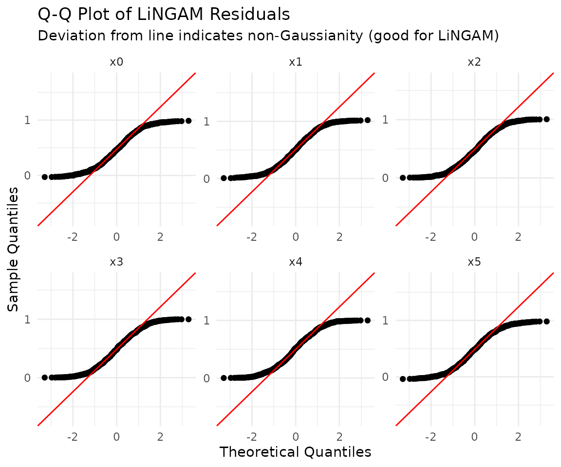
If normality is not rejected, the causal direction may be unidentifiable — see the non-Gaussianity experiments in the Direct LiNGAM article.
Model Summary
summary_lingam() runs the residual independence test and
the normality test together, letting you review at a glance how well the
two assumptions LiNGAM relies on hold (that the residuals are mutually
independent, and that the residuals are non-Gaussian). Instead of
calling get_error_independence_p_values() and
test_residual_normality() separately, you can survey the
diagnostics in one place.
x1k$data |>
  summary_lingam(model)
#> === Direct LiNGAM Model Summary ===
#> Variables:    6
#> Observations: 1000
#> Edges:        7
#> Causal order: x3 -> x2 -> x0 -> x4 -> x5 -> x1
#>
#> --- Assumption 1: Independence of residuals ---
#> Method:           spearman
#> Dependent pairs:  0 / 15  (p < 0.050)
#> Min p-value:      0.0510
#> => Residuals appear mutually independent (assumption supported).
#>
#> --- Assumption 2: Non-Gaussianity of residuals ---
#> Method:           shapiro
#> Non-Gaussian:     6 / 6  (p <= 0.050)
#> => All residuals are non-Gaussian (assumption supported).
Bootstrap Direct LiNGAM
We assess the reliability of the model using the bootstrap method.
bs_model <- x1k$data |>
  lingam_direct_bootstrap(n_sampling = 100L, seed = 42)
#> Bootstrap: 100 iterations, method=adaptive_lasso (sequential)
#>   iteration 1 / 100
#>   iteration 10 / 100
#>   iteration 20 / 100
#>   iteration 30 / 100
#>   iteration 40 / 100
#>   iteration 50 / 100
#>   iteration 60 / 100
#>   iteration 70 / 100
#>   iteration 80 / 100
#>   iteration 90 / 100
#>   iteration 100 / 100
#> Completed in 3.2 seconds.

bs_model
#> BootstrapResult: 100 samplings, 6 features
When the number of iterations or variables is large, specifying
parallel = TRUE lets it run faster on multiple cores. The
number of cores is specified with n_cores (when
unspecified, it is capped at 2 cores for safety).
bs_model <- x1k$data |>
  lingam_direct_bootstrap(
    n_sampling = 100L,
    seed       = 42,
    parallel   = TRUE,
    n_cores    = 4L
  )
Note that parallel execution uses L’Ecuyer’s parallel random number
streams, so results are reproducible given the same seed
and the same n_cores, but they will not numerically match
the results of sequential execution (parallel = FALSE).
Inspecting the Bootstrap Results
From the bootstrap results, we compute the frequency of occurrence of each path and the mean of the coefficients.
bs_model |>
  get_causal_direction_counts(labels = names(x1k$data))
#>    from to count proportion mean_effect median_effect  sd_effect    ci_lower
#> 1     1  6   100       1.00  4.01532920    4.01513886 0.01126767  3.99550980
#> 2     1  2    99       0.99  2.98181621    2.97864538 0.02849338  2.92980702
#> 3     1  5    99       0.99  8.00994011    8.00748238 0.02951185  7.95680521
#> 4     3  2    99       0.99  2.00498455    2.00660933 0.01479861  1.97675886
#> 5     3  5    99       0.99 -1.00529230   -1.00485827 0.01523485 -1.03801290
#> 6     4  1    99       0.99  3.03521019    3.03586526 0.03001961  2.97855949
#> 7     4  3    99       0.99  5.99644109    5.99745219 0.03186571  5.94050363
#> 8     2  1     1       0.01  0.05304916    0.05304916 0.00000000  0.05304916
#> 9     2  3     1       0.01  0.40196452    0.40196452 0.00000000  0.40196452
#> 10    2  5     1       0.01  0.90679690    0.90679690 0.00000000  0.90679690
#> 11    3  4     1       0.01  0.16166764    0.16166764 0.00000000  0.16166764
#> 12    5  1     1       0.01  0.10453910    0.10453910 0.00000000  0.10453910
#> 13    5  3     1       0.01 -0.13636255   -0.13636255 0.00000000 -0.13636255
#>       ci_upper from_name to_name
#> 1   4.03698551        x0      x5
#> 2   3.03860193        x0      x1
#> 3   8.07414013        x0      x4
#> 4   2.03193816        x2      x1
#> 5  -0.97488336        x2      x4
#> 6   3.09304642        x3      x0
#> 7   6.06134091        x3      x2
#> 8   0.05304916        x1      x0
#> 9   0.40196452        x1      x2
#> 10  0.90679690        x1      x4
#> 11  0.16166764        x2      x3
#> 12  0.10453910        x4      x0
#> 13 -0.13636255        x4      x2
Adjacency Matrix of Mean Causal Effects
We construct an adjacency matrix from the bootstrap results.
bs_adjacency_matrix <- bs_model |>
  get_adjacency_matrix_summary(stat = "median")

bs_adjacency_matrix |>
  round(3)
#>       [,1]  [,2]   [,3]  [,4]   [,5] [,6]
#> [1,] 0.000 0.053  0.000 3.036  0.105    0
#> [2,] 2.979 0.000  2.007 0.000  0.000    0
#> [3,] 0.000 0.402  0.000 5.997 -0.136    0
#> [4,] 0.000 0.000  0.162 0.000  0.000    0
#> [5,] 8.007 0.907 -1.005 0.000  0.000    0
#> [6,] 4.015 0.000  0.000 0.000  0.000    0
We visualize the estimated adjacency matrix.
bs_adjacency_matrix |>
  plot_adjacency(
    labels    = colnames(x1k$data),
    title     = "Estimated (with Bootstrap)",
    rankdir   = "TB",
    shape     = "circle",
    fillcolor = "lightgreen"
  )
Matrix of Path Occurrence Frequencies
We compute the matrix of occurrence frequencies for each path.
bs_model |>
  get_probabilities()
#>      [,1] [,2] [,3] [,4] [,5] [,6]
#> [1,] 0.00 0.01 0.00 0.99 0.01    0
#> [2,] 0.99 0.00 0.99 0.00 0.00    0
#> [3,] 0.00 0.01 0.00 0.99 0.01    0
#> [4,] 0.00 0.00 0.01 0.00 0.00    0
#> [5,] 0.99 0.01 0.99 0.00 0.00    0
#> [6,] 1.00 0.00 0.00 0.00 0.00    0
Mean Total Effects
We compute the mean total effect of each path.
bs_model |>
  get_total_causal_effects()
#>    from to      effect probability
#> 1     1  6  4.01520158        1.00
#> 2     1  2  2.87431611        0.99
#> 3     1  5  7.90813117        0.99
#> 4     3  2  1.95874622        0.99
#> 5     3  5 -1.06193484        0.99
#> 6     4  1  3.03586526        0.99
#> 7     4  2 21.07027271        0.99
#> 8     4  3  5.99805118        0.99
#> 9     4  5 18.28272145        0.99
#> 10    4  6 12.18719857        0.99
#> 11    3  6 -0.24574320        0.04
#> 12    2  1  0.14794503        0.01
#> 13    2  3  0.27850920        0.01
#> 14    2  4  0.04611007        0.01
#> 15    2  5  0.90679690        0.01
#> 16    2  6  0.59359217        0.01
#> 17    3  4  0.16192779        0.01
#> 18    5  1  0.10498716        0.01
#> 19    5  3 -0.13625059        0.01
#> 20    5  6  0.42156703        0.01
#> 21    6  2  0.24518629        0.01
We turn the bootstrap results into a causal graph. By default, only paths that occur in at least 50% of samples are shown.
bs_model |>
  plot_bootstrap_probabilities()
Paths Between Two Variables
get_paths() breaks the total causal effect between two
variables down into the individual paths that carry it, along with each
path’s bootstrap probability. As shown in the Direct LiNGAM article, the true structure
of generate_lingam_sample_6() has two paths from x3 to x1:
x3 -> x0 -> x1 (indirect effect 9.0) and
x3 -> x2 -> x1 (indirect effect 12.0). Indices are
1-based, so x3 (column 4) to x1 (column 2) is:
bs_model |>
  get_paths(4, 2)
#>      path    effect probability
#> 1 4, 1, 2  9.041187        0.99
#> 2 4, 3, 2 12.020020        0.99
Both paths are recovered in 99 of the 100 bootstrap samples, with median effects close to the true values (9.0 and 12.0).
Frequency of Recurring DAG Structures
get_directed_acyclic_graph_counts() looks at the whole
graph estimated in each bootstrap sample and counts how often each
distinct DAG — rather than individual edges — recurs.
n_dags limits the output to the most frequent
structures.
dag_counts <- bs_model |>
  get_directed_acyclic_graph_counts(n_dags = 3)

dag_counts$count
#> [1] 99  1

dag_counts$dag[[1]]
#>   from to
#> 1    1  2
#> 2    1  5
#> 3    1  6
#> 4    3  2
#> 5    3  5
#> 6    4  1
#> 7    4  3
The most frequent DAG (99 of the 100 samples) matches the true edge
set of generate_lingam_sample_6() exactly.
Stability of the Causal Order
get_causal_order_stability() aggregates the causal
orders estimated in each bootstrap sample and quantifies how stable the
order is. It returns the rank distribution of each variable, the
precedence probability for variable pairs (P[i, j] = the
fraction of samples in which variable i came upstream of j), and an
overall stability score (0 = random, 1 = identical across all
samples).
bs_model |>
  get_causal_order_stability(labels = names(x1k$data))
#> === Causal Order Stability ===
#> Bootstrap samples:       100
#> Overall stability score: 0.736  (0 = random, 1 = fully stable)
#>
#> Rank summary (sorted by mean rank; 1 = most upstream):
#>  variable mean_rank sd_rank median_rank mode_rank
#>        x3      1.05    0.50           1         1
#>        x0      2.62    0.51           3         3
#>        x2      2.75    0.95           2         2
#>        x5      4.41    1.23           4         3
#>        x4      4.92    0.77           5         5
#>        x1      5.25    0.88           5         6
#>
#> Precedence probability P[i, j] = P(variable i precedes j):
#>      x0   x1   x2   x3   x4   x5
#> x0 0.00 0.99 0.39 0.01 0.99 1.00
#> x1 0.01 0.00 0.01 0.01 0.38 0.34
#> x2 0.61 0.99 0.00 0.01 0.99 0.65
#> x3 0.99 0.99 0.99 0.00 0.99 0.99
#> x4 0.01 0.62 0.01 0.01 0.00 0.43
#> x5 0.00 0.66 0.35 0.01 0.57 0.00
Caveat: bootstrap stability does not guarantee correctness. When a model assumption is violated, the wrong structure can be reproduced stably — see the measurement error paradox in the Direct LiNGAM article for a worked example.
Evaluating Model Fit
evaluate_model_fit() treats an estimated adjacency
matrix as a structural equation model (SEM) and reports standard SEM fit
measures (CFI, RMSEA, AIC/BIC, etc.) via the lavaan package
(an optional dependency; install it with
install.packages("lavaan")). This is useful for judging
whether an estimated causal graph is consistent with the data,
independent of how it was estimated.
sample6 <- generate_lingam_sample_6()
fit_result <- lingam_direct(sample6$data, reg_method = "ols")

# fit measures for the estimated graph
evaluate_model_fit(fit_result, sample6$data)
#>   DoF DoF Baseline chi2 chi2 p-value chi2 Baseline CFI GFI AGFI NFI TLI RMSEA
#> 1   0           15    0           NA       23023.7   1   1   NA   1   1     0
#>        AIC      BIC    LogLik
#> 1 1860.598 1958.753 -910.2991
Reversing the direction of every edge produces a mis-specified model, and its fit measures are visibly worse (lower CFI, higher RMSEA):
reversed_adjacency <- t(fit_result$adjacency_matrix)
evaluate_model_fit(reversed_adjacency, sample6$data)
#>   DoF DoF Baseline         chi2 chi2 p-value chi2 Baseline CFI GFI AGFI NFI TLI
#> 1   0           15 2.664535e-11           NA       23023.7   1   1   NA   1   1
#>   RMSEA       AIC       BIC   LogLik
#> 1     0 -4264.864 -4166.708 2152.432
Integration with broom (tidy / glance)
Estimation results can be converted to a data.frame with the
broom-compatible tidy() /
glance(), making integration with ggplot2 and
dplyr easy. tidy() returns an edge list
(from, to, estimate), and
glance() returns a one-row summary of the whole model.
tidy() also works on bootstrap results, in which case it
returns the occurrence frequencies for each direction, etc.
# Convert the estimated adjacency matrix to an edge list
tidy(model)
#>   from to  estimate
#> 1   x0 x1  2.987705
#> 2   x0 x4  8.000096
#> 3   x0 x5  4.014962
#> 4   x2 x1  2.001708
#> 5   x2 x4 -1.000306
#> 6   x3 x0  3.032952
#> 7   x3 x2  5.992677

# One-row summary of the whole model
glance(model)
#>   n_variables n_edges                     causal_order
#> 1           6       7 x3 -> x2 -> x0 -> x4 -> x5 -> x1

# Direction-wise summary of the bootstrap results (variable names via labels)
tidy(bs_model, labels = names(x1k$data))
#>    from to count proportion mean_effect median_effect  sd_effect    ci_lower
#> 1     1  6   100       1.00  4.01532920    4.01513886 0.01126767  3.99550980
#> 2     1  2    99       0.99  2.98181621    2.97864538 0.02849338  2.92980702
#> 3     1  5    99       0.99  8.00994011    8.00748238 0.02951185  7.95680521
#> 4     3  2    99       0.99  2.00498455    2.00660933 0.01479861  1.97675886
#> 5     3  5    99       0.99 -1.00529230   -1.00485827 0.01523485 -1.03801290
#> 6     4  1    99       0.99  3.03521019    3.03586526 0.03001961  2.97855949
#> 7     4  3    99       0.99  5.99644109    5.99745219 0.03186571  5.94050363
#> 8     2  1     1       0.01  0.05304916    0.05304916 0.00000000  0.05304916
#> 9     2  3     1       0.01  0.40196452    0.40196452 0.00000000  0.40196452
#> 10    2  5     1       0.01  0.90679690    0.90679690 0.00000000  0.90679690
#> 11    3  4     1       0.01  0.16166764    0.16166764 0.00000000  0.16166764
#> 12    5  1     1       0.01  0.10453910    0.10453910 0.00000000  0.10453910
#> 13    5  3     1       0.01 -0.13636255   -0.13636255 0.00000000 -0.13636255
#>       ci_upper from_name to_name
#> 1   4.03698551        x0      x5
#> 2   3.03860193        x0      x1
#> 3   8.07414013        x0      x4
#> 4   2.03193816        x2      x1
#> 5  -0.97488336        x2      x4
#> 6   3.09304642        x3      x0
#> 7   6.06134091        x3      x2
#> 8   0.05304916        x1      x0
#> 9   0.40196452        x1      x2
#> 10  0.90679690        x1      x4
#> 11  0.16166764        x2      x3
#> 12  0.10453910        x4      x0
#> 13 -0.13636255        x4      x2
Related Articles
- Method selection guide
- Direct LiNGAM in depth — including the measurement error paradox, where the bootstrap is stably wrong
- Time series, latent confounders, special data — each method’s own bootstrap variant