Gains and lift table for a CHAID tree

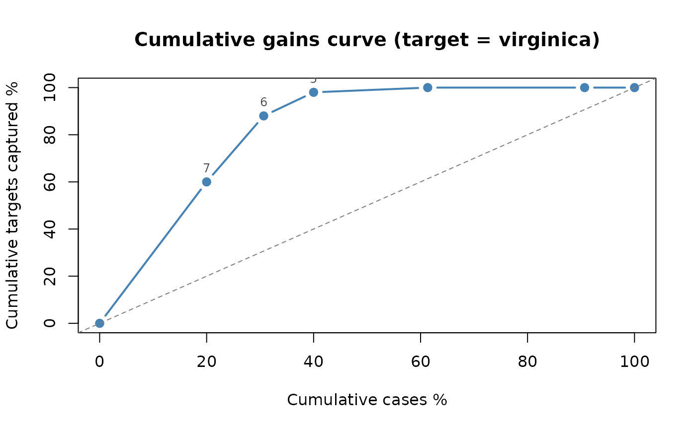
Sorts the terminal nodes by decreasing response rate (node mean for continuous responses) and computes cumulative gains and lift, corresponding to the SPSS gains table.

Usage

chaid_gains(fit, data = NULL, target = NULL, weights = NULL, freq = NULL)

# S3 method for class 'chaid_gains'
print(x, ...)

# S3 method for class 'chaid_gains'
plot(x, type = c("gains", "lift"), ...)

Arguments

fit

A fitted "chaid" object returned by chaid().

data

Optional data frame. If NULL (default), node statistics from training are used. If supplied, cases are routed with predict.chaid() and the table is recomputed, e.g. for evaluation on holdout data.

target

Response level of interest for categorical responses. For a binary response the second level is used by default; for three or more levels target is required.

weights, freq

Case and frequency weights for data, when supplied.

x

A "chaid_gains" object.

...

For plot(), further arguments passed to graphics::plot(); ignored by print().

type

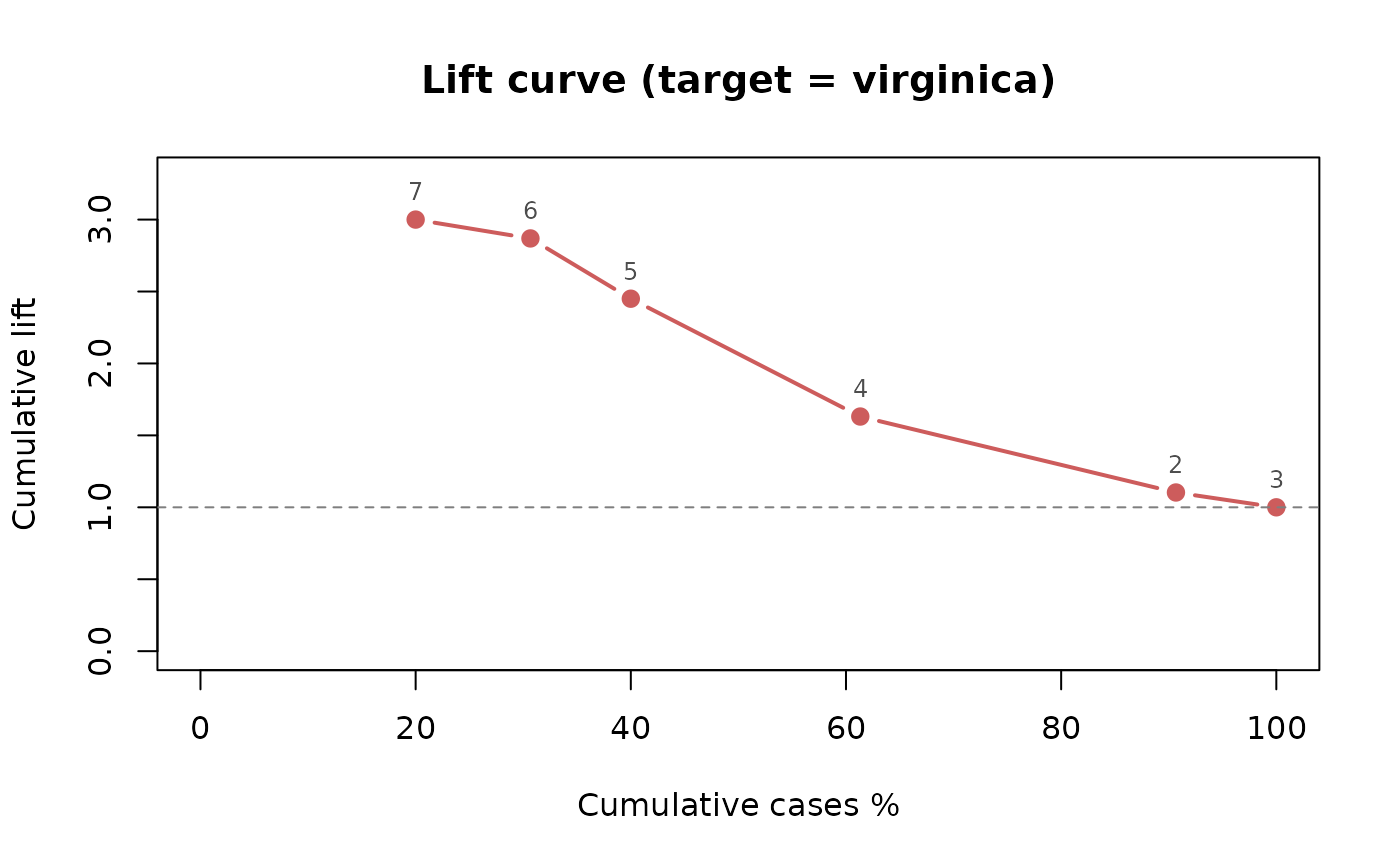
"gains" (default) draws the cumulative gains curve (percentage of cases vs. percentage of captured targets, diagonal = random), "lift" draws the cumulative lift curve (1 = random).

Value

An object of class "chaid_gains", a list with the gains table (table), the target level, the response type (ytype), the overall rate (overall) and the data source ("training" or "newdata"). print() and plot() methods are available.

See also

chaid_table(), chaid_validate()

Examples

fit <- chaid(Species ~ ., data = iris,
             control = chaid_control(min_parent = 30, min_child = 10))
g <- chaid_gains(fit, target = "virginica")
print(g)
#> CHAID gains table (target = virginica) 
#> Overall response rate: 0.3333 
#> 
#>  node  n pct_n resp pct_resp   rate index cum_pct_n cum_pct_resp cum_lift
#>     7 30 20.00   30       60 1.0000 300.0     20.00           60    3.000
#>     6 16 10.67   14       28 0.8750 262.5     30.67           88    2.869
#>     5 14  9.33    5       10 0.3571 107.1     40.00           98    2.450
#>     4 32 21.33    1        2 0.0312   9.4     61.33          100    1.631
#>     2 44 29.33    0        0 0.0000   0.0     90.67          100    1.103
#>     3 14  9.33    0        0 0.0000   0.0    100.00          100    1.000
plot(g)

plot(g, type = "lift")